Literature
Display
← All papers

MCP: Learning Composable Hierarchical Control with Multiplicative Compositional Policies

Xue Bin Peng · Michael Chang · Grace Zhang · Pieter Abbeel · Sergey Levine

· NeurIPS 2019 ↗

Robotics7 min text · CondensedOriginal paper ↗
Contents

At a glance

MCP represents a policy as a weighted product of learned Gaussian motor primitives. Several primitives influence each action simultaneously, allowing new combinations after pretraining. A new gating policy learns how to combine frozen primitives for a transfer task.

Experiments use simulated ants, bipeds, humanoids, and a T-Rex. The largest gains appear on difficult locomotion-and-manipulation tasks; the results depend on useful motion-imitation pretraining and do not show physical robot deployment.

1 Introduction

Relearning each task from scratch wastes useful motor experience. Temporal skill selection activates one behavior at a time; MCP instead combines primitives within the current action distribution. This creates a continuous control space that a transfer policy can explore while retaining the pretrained motor representation.

2 Preliminaries

Pretraining and transfer tasks share states, actions, and dynamics, while goals and rewards may differ. Transfer assumes some relevant shared skills. An additive mixture samples one primitive before sampling an action; MCP’s product combines contributions before drawing the action.

Equation 1
π⁡(a|s,g)=∑i=1kwi​(s,g)​πi​(a|s,g),∑i=1kwi​(s,g)=1,wi​(s,g)≥0.\pi(a|s,g)=\sum_{i=1}^{k}w_{i}(s,g)\pi_{i}(a|s,g),\quad\sum_{i=1}^{k}w_{i}(s,g)=1,\quad w_{i}(s,g)\geq 0. (1)

3 Multiplicative Compositional Policies

Each primitive supplies an action density, raised to a nonnegative gating weight. Multiplication and normalization produce the composite density. Weights need not sum to one; experiments bound them between zero and one.

Equation 2
π⁡(a|s,g)=1Z⁡(s,g)​∏i=1kπi​(a|s,g)wi​(s,g),wi​(s,g)≥0.\pi(a|s,g)=\frac{1}{Z(s,g)}\prod_{i=1}^{k}\pi_{i}(a|s,g)^{w_{i}(s,g)},\quad w_{i}(s,g)\geq 0. (2)

3.1 Gaussian Primitives

A product of diagonal Gaussian primitives is another diagonal Gaussian. Its mean uses precision-weighted primitive means, and its precision sums the weighted primitive precisions. Consequently, both the gate and each primitive’s uncertainty determine influence on each action coordinate. This closed form supports ordinary end-to-end policy optimization.

Equation 3
μj(s,g)=1∑l=1kwl​(s,g)σlj​(s,g)∑i=1kwi​(s,g)σij​(s,g)μij(s,g),σj(s,g)=(∑i=1kwi​(s,g)σij​(s,g))−1.\displaystyle\mu^{j}(s,g)=\frac{1}{\sum_{l=1}^{k}\frac{w_{l}(s,g)}{\sigma_{l}^{j}(s,g)}}\sum_{i=1}^{k}\frac{w_{i}(s,g)}{\sigma_{i}^{j}(s,g)}\mu_{i}^{j}(s,g),\qquad\sigma^{j}(s,g)=\left(\sum_{i=1}^{k}\frac{w_{i}(s,g)}{\sigma_{i}^{j}(s,g)}\right)^{-1}. (3)

3.2 Pre-Training and Transfer

All primitives train jointly across pretraining tasks. Only the gate sees the goal; primitives see state, encouraging reusable behavior rather than a goal-specific controller inside every primitive. At transfer, primitive parameters are frozen and a new gate learns composition weights. The original algorithm gives both stages.

Algorithm 1 MCP Pre-Training and Transfer
1:  Pre-training:
2:  πi←\pi_{i}\leftarrow random parameters for i=1,…,ki=1,...,k
3:  w←w\leftarrow random parameters
4:  π1:k∗,w∗=arg maxπ1:k,wJp​r​e(π1:k,w)\pi_{1:k}^{*},w^{*}=\underset{\pi_{1:k},w}{\text{arg max}}\ \ J_{pre}\left(\pi_{1:k},w\right)
5:  Transfer:
6:  ω←\omega\leftarrow random parameters
7:  ω∗=arg max𝜔Jt​r​a(π1:k∗,ω)\omega^{*}=\underset{\omega}{\text{arg max}}\ \ J_{tra}\left(\pi_{1:k}^{*},\omega\right)
Equation 4
π⁡(a|s,g)=1Z⁡(s,g)​∏i=1kπi​(a|s)wi​(s,g),πi​(a|s)=𝒩⁡(μi​(s),Σi​(s)).\pi(a|s,g)=\frac{1}{Z(s,g)}\prod_{i=1}^{k}\pi_{i}(a|s)^{w_{i}(s,g)},\quad\pi_{i}(a|s)=\mathcal{N}\left(\mu_{i}(s),\Sigma_{i}(s)\right). (4)

4 Related Work

The approach relates to transfer learning, hierarchical policies, and continuous latent skill spaces. Freezing primitives preserves their learned parameters while allowing the new gate to repurpose them.

Hierarchical Policies:

Hierarchical methods typically learn or pretrain low-level skills and select among them over time. MCP’s comparison asks whether simultaneous composition provides a richer range of actions than selecting one skill at a time.
Refer to caption
(a) Ant
Refer to caption
(b) Biped
Refer to caption
(c) Humanoid
Refer to caption
(d) T-Rex
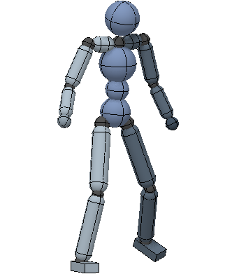
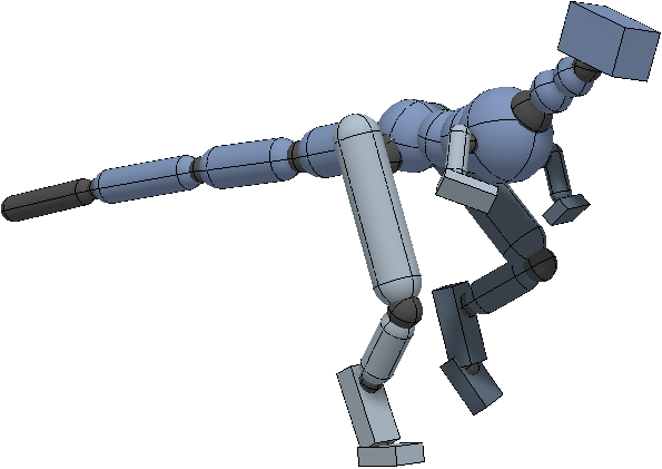
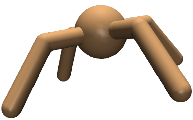
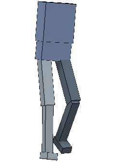
Figure 1: Our method is evaluated on complex 3D characters with different morphologies and large numbers of degrees-of-freedom.

Latent Space Models:

Continuous latent models map a code into motor actions. [14] MCP gives that code explicit structure as primitive-composition weights. The proposed benefit is a reusable action representation whose combinations remain flexible on new goals.

5 Experiments

The benchmark uses a 14-degree-of-freedom ant, 23-degree-of-freedom biped, 34-degree-of-freedom humanoid, and 55-degree-of-freedom T-Rex. Tests combine locomotion, balance, object transport, and ball manipulation in simulation.

5.1 Experimental Setup

The protocol first learns imitation skills, then trains transfer controllers on new rewards.

Pre-Training Tasks:

Pretraining tracks walking and turning motion clips. The gate receives the next two target states. Random clip changes during an episode encourage transitions between skills; the primitives remain state-conditioned.
Refer to caption
(a) Heading: Humanoid
Refer to caption
(b) Carry: Biped
Refer to caption
(c) Dribble: Humanoid
Refer to caption
(d) Dribble: T-Rex
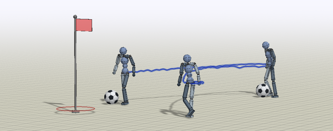
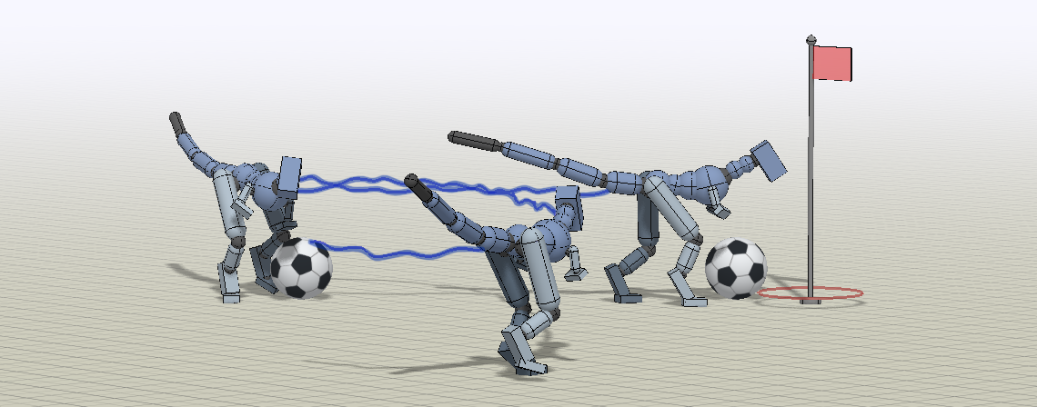
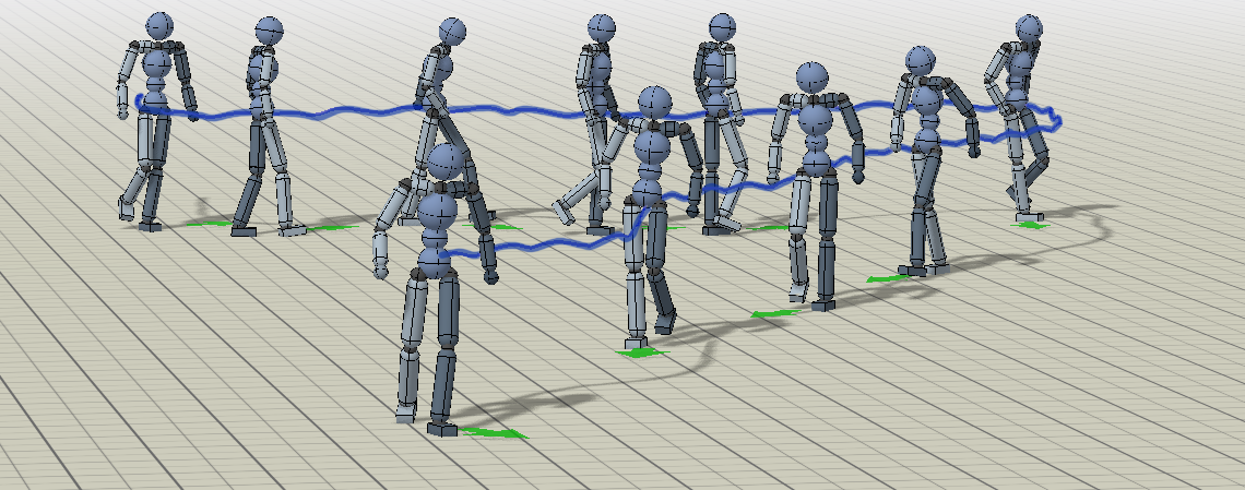
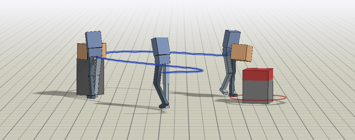
Figure 2: The transfer tasks pose a challenging combination of locomotion and object manipulation, such as carrying an object to a target location and dribbling a ball to a goal, which requires coordination of multiple body parts and temporally extended behaviors.

Transfer Tasks:

Heading follows a changing direction. Carry picks up a box, transports it, and places it at a target; the simulator attaches the box through a virtual joint after designated contact. Dribble moves a ball to a target through contact while maintaining balance. Goal inputs provide relevant object and target state.
Refer to caption
Refer to caption
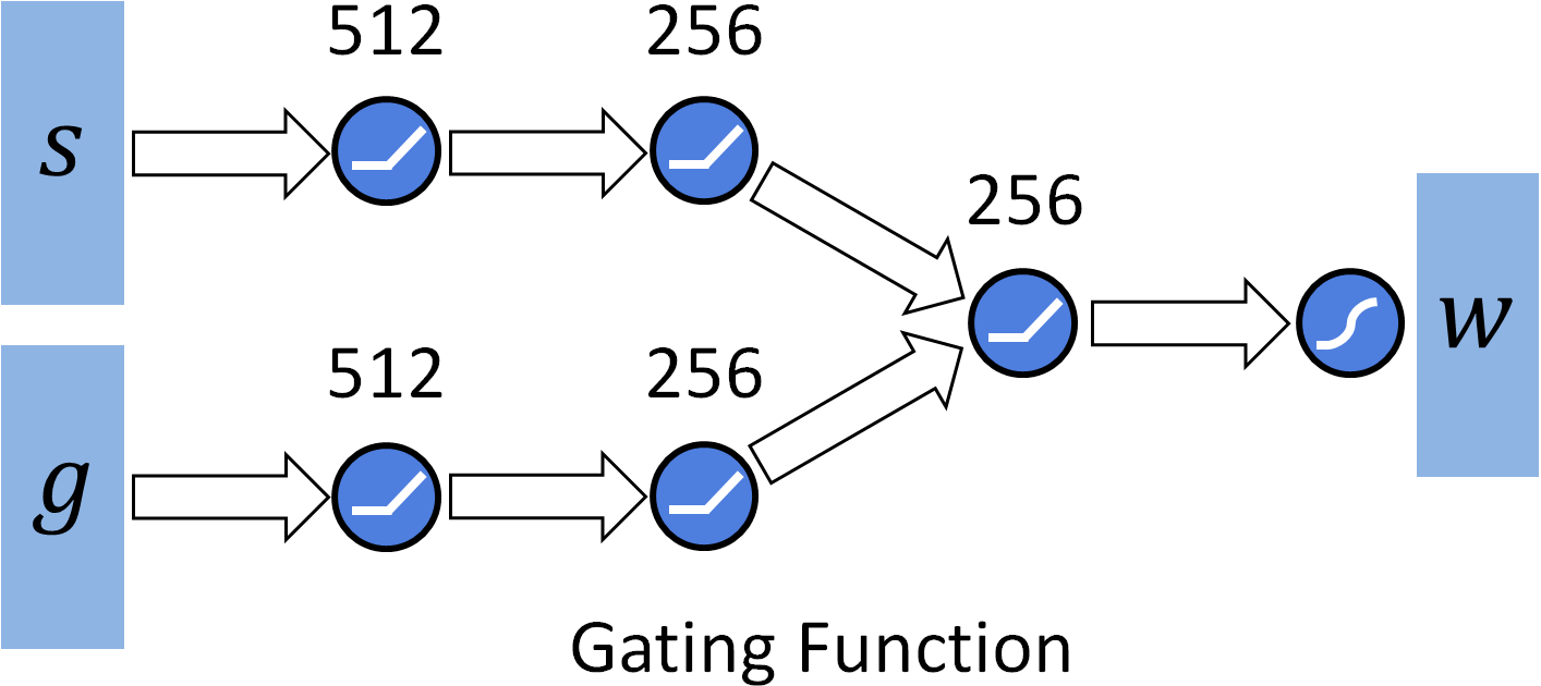
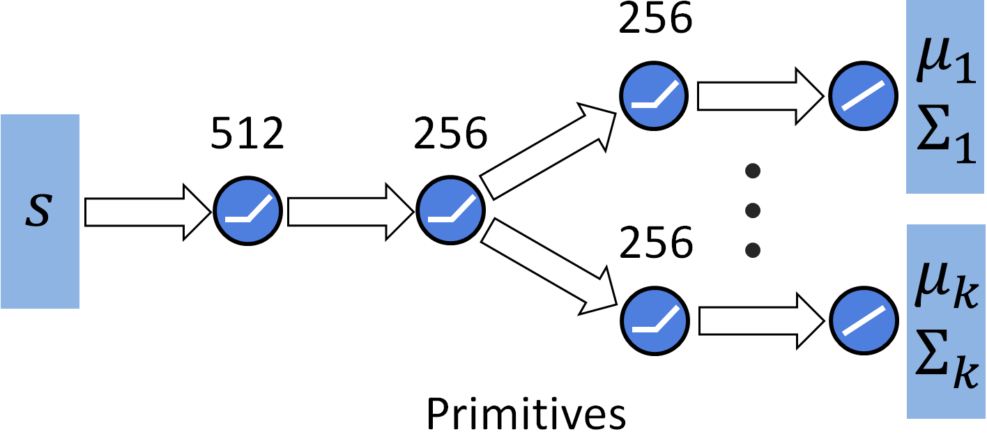
Figure 3: Schematic illustrations of the MCP architecture. The gating function receives both ss and gg as inputs, which are first encoded by separate networks, with 512 and 256 units. The resulting features are concatenated and processed with a layer of 256 units, followed by a sigmoid output layer to produce the weights w⁡(s,g)w(s,g). The primitives receive only ss as input, which is first processed by a common network, with 512 and 256 units, before branching into separate layers of 256 units for each primitive, followed by a linear output layer that produces μi​(s)\mu_{i}(s) and Σi​(s)\Sigma_{i}(s) for each primitive. ReLU activation is used for all hidden units.
Environment Scratch Finetune Hierarchical Option-Critic MOE Latent Space MCP (Ours)
Heading: Biped 0.927±0.0320.927\pm 0.032 0.970±0.0020.970\pm 0.002 0.834±0.0010.834\pm 0.001 0.952±0.0120.952\pm 0.012 0.918±0.0020.918\pm 0.002 0.970±0.0010.970\pm 0.001 0.976±0.002\bf{0.976\pm 0.002}
Carry: Biped 0.027±0.0350.027\pm 0.035 0.324±0.0140.324\pm 0.014 0.001±0.0020.001\pm 0.002 0.346±0.0110.346\pm 0.011 0.013±0.0130.013\pm 0.013 0.456±0.0310.456\pm 0.031 0.575±0.032\bf{0.575\pm 0.032}
Dribble: Biped 0.072±0.0120.072\pm 0.012 0.651±0.0250.651\pm 0.025 0.546±0.0240.546\pm 0.024 0.046±0.0080.046\pm 0.008 0.073±0.0210.073\pm 0.021 0.768±0.0120.768\pm 0.012 0.782±0.008\bf{0.782\pm 0.008}
Dribble: Humanoid 0.076±0.0240.076\pm 0.024 0.598±0.0300.598\pm 0.030 0.198±0.0020.198\pm 0.002 0.058±0.0070.058\pm 0.007 0.043±0.0210.043\pm 0.021 0.751±0.0060.751\pm 0.006 0.805±0.006\bf{0.805\pm 0.006}
Dribble: T-Rex 0.065±0.0320.065\pm 0.032 0.074±0.0110.074\pm 0.011 −- 0.098±0.0130.098\pm 0.013 0.070±0.0170.070\pm 0.017 0.115±0.0130.115\pm 0.013 0.781±0.021\bf{0.781\pm 0.021}
Holdout: Ant 0.951±0.093\bf{0.951\pm 0.093} 0.885±0.0620.885\pm 0.062 −- −- −- 0.745±0.0600.745\pm 0.060 0.812±0.0300.812\pm 0.030
Table 1: Performance statistics of different models on transfer tasks. Additional experiments are available in the supplementary material. MCP outperforms other methods on a suite of challenging tasks with complex simulated characters.

Model Representation:

The main model has eight primitives and separate gate and primitive networks. State includes body-relative link poses and velocities; actions specify joint PD targets at 30 Hz. PPO trains the policies, with the full network structure retained in Figure 3. [34]

5.2 Comparisons

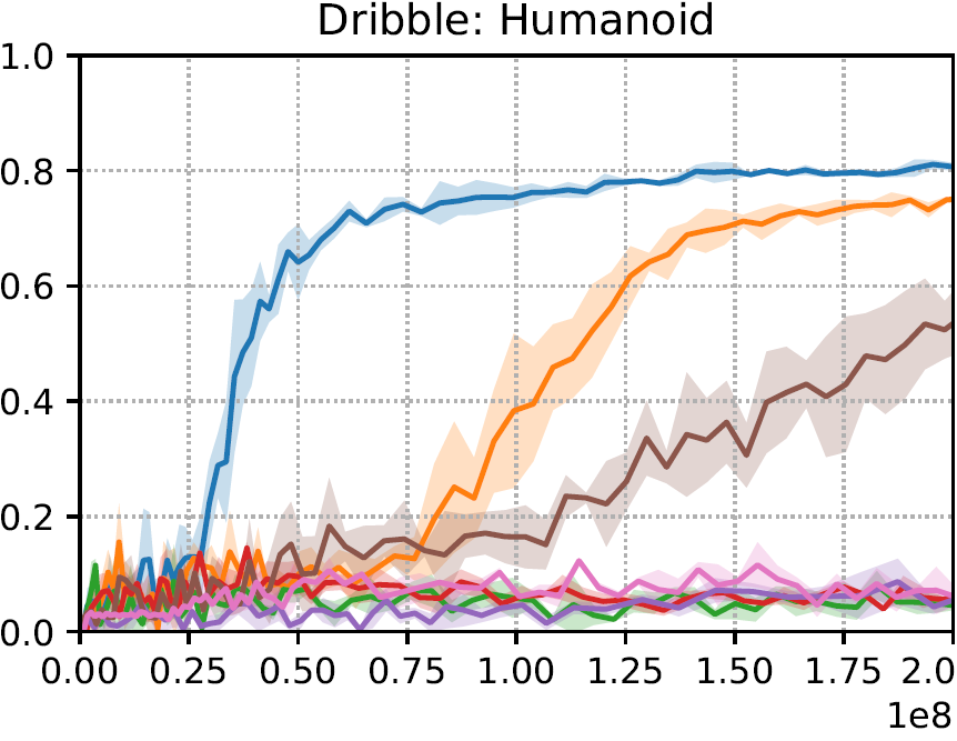
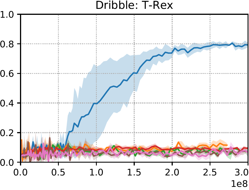
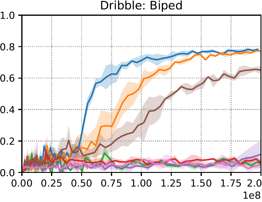
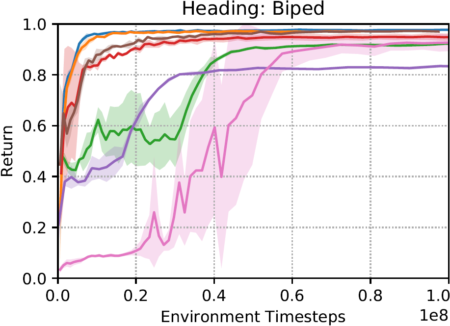
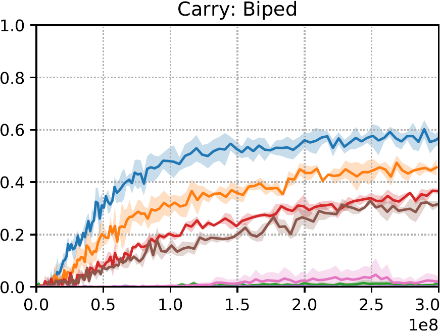
Three seeds per method and environment are evaluated over about 100 episodes each. Scores are normalized returns, not success percentages. MCP reaches 0.575 on biped carrying versus 0.456 for the latent model, 0.805 versus 0.751 on humanoid dribbling, and 0.781 versus 0.115 on T-Rex dribbling. It is the only tested model reported to solve the latter task.

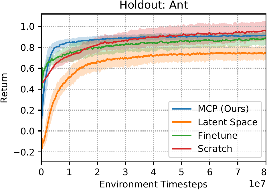
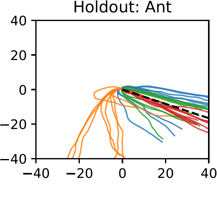
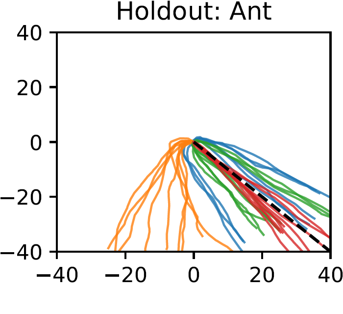
Benefits are not universal: heading is easier for several baselines, and scratch training scores 0.951 on held-out ant directions versus MCP’s 0.812. The authors attribute MCP’s harder-task gains partly to flexible combinations of primitives, while latent decoders can overfit pretraining behaviors.
Refer to caption
Refer to caption
Refer to caption
Refer to caption
Refer to caption
Figure 4: Learning curves of the various models when applied to transfer tasks. MCP substantially improves learning speed and performance on challenging tasks (e.g. carry and dribble), and is the only method that succeeds on the most difficult task (Dribble: T-Rex).
Refer to caption
Refer to caption
Refer to caption
Refer to caption
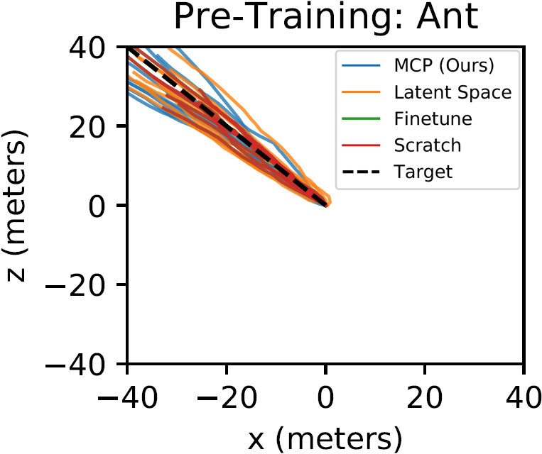
Figure 5: Left: Learning curves on holdout tasks in the Ant environment. Right: Trajectories produced by models with target directions from pre-training, and target directions from the holdout set after training on transfer tasks. The latent space model is prone to overfitting to the pre-training tasks, and can struggle to adapt to the holdout tasks.
Refer to caption
Refer to caption
Refer to caption
Refer to caption
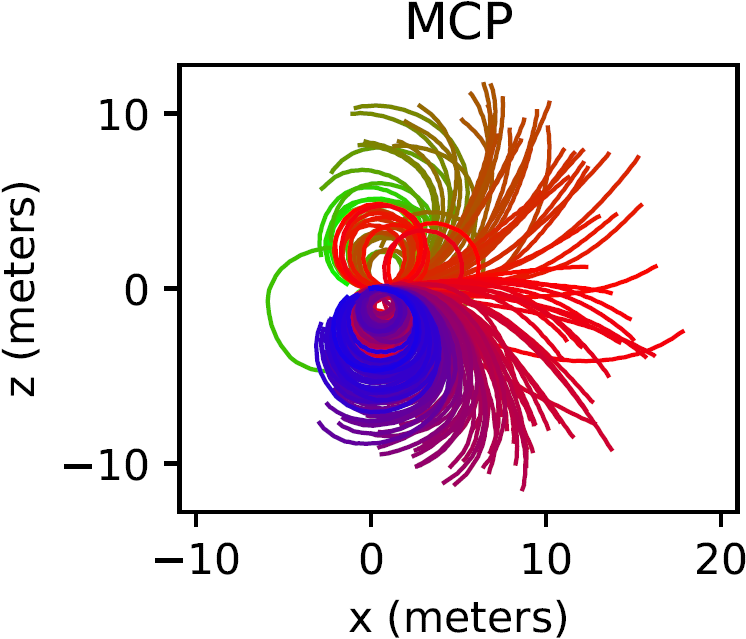
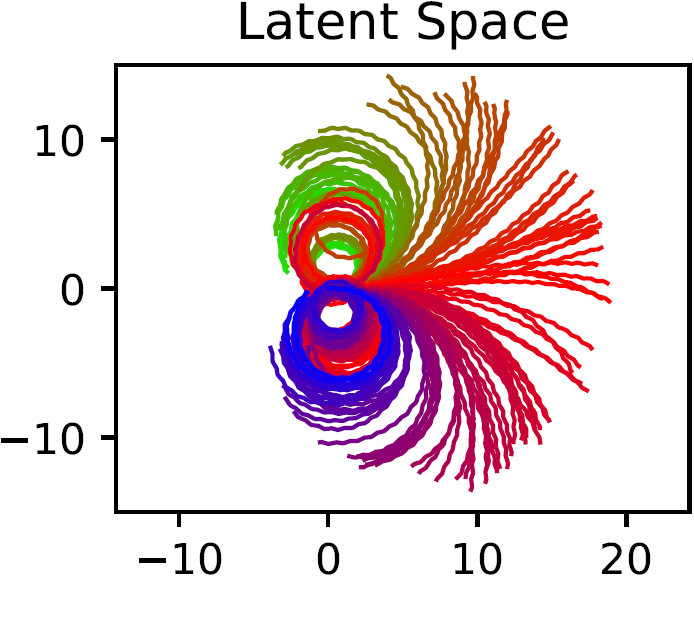
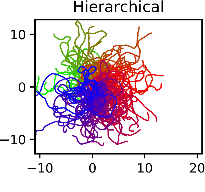
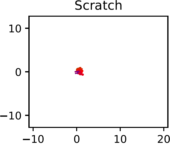
Figure 6: Trajectories of the humanoid’s root along the horizontal plane visualizing the exploration behaviors of different models. MCP and other models that are pre-trained with motion imitation produce more structured exploration behaviors.
Refer to caption
Refer to caption
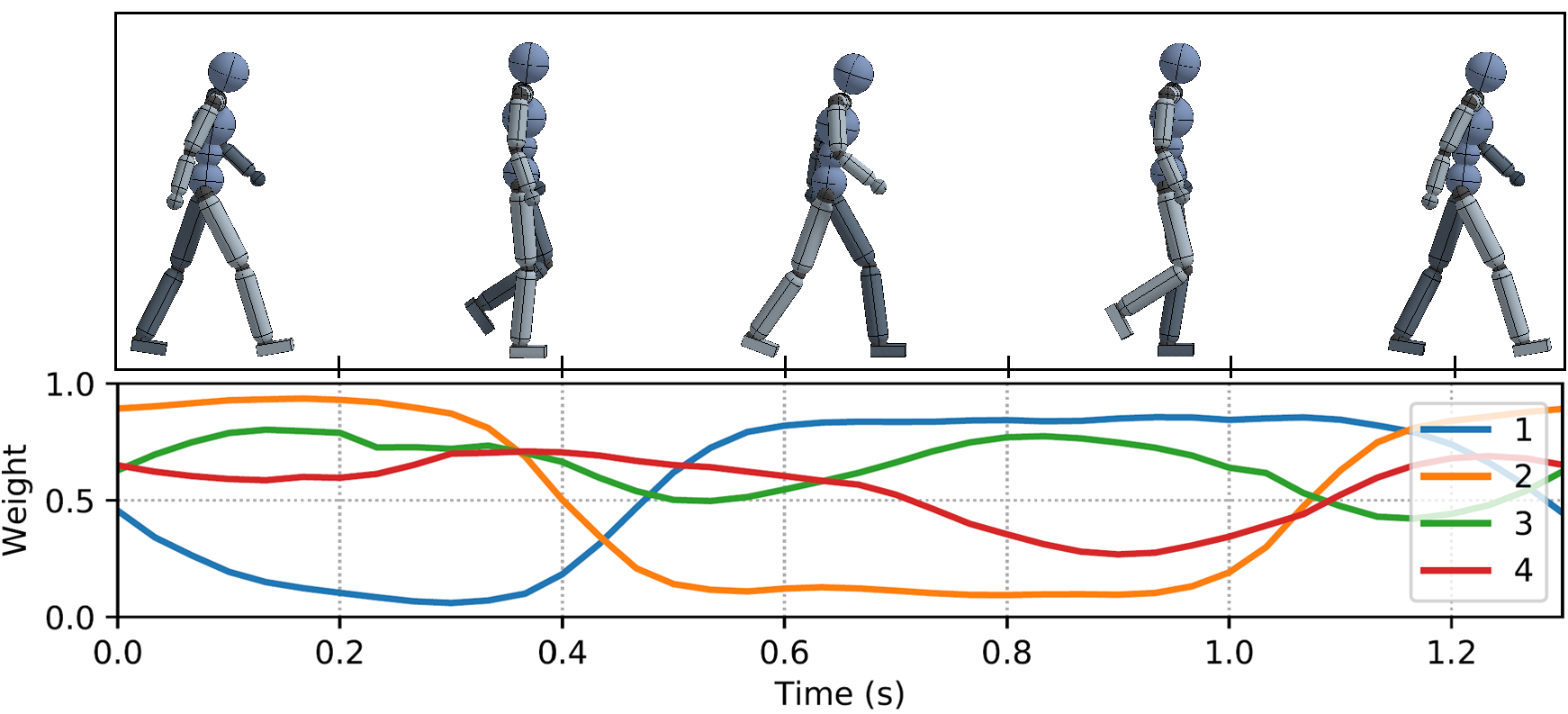
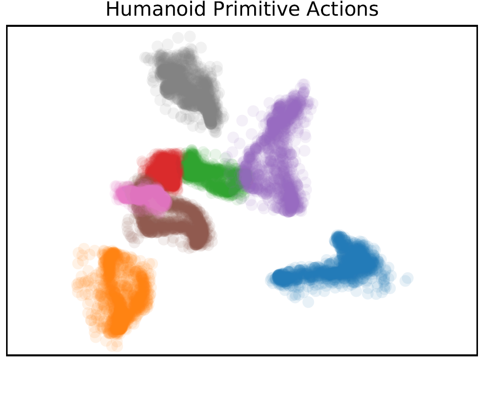
Figure 7: Left: Weights for primitives over the course of a walk cycle. Primitives develop distinct specializations, with some primitives becoming most active during the left stance phase, and others during right stance. Right: PCA embedding of actions from each primitive exhibits distinct clusters.

5.3 Exploration Behaviors

Randomly combining pretrained primitives produces coherent motion in different directions. Direct independent action noise instead makes the humanoid fall quickly. Latent and hierarchical pretraining also improve exploration, so structured exploration is not unique to MCP.

5.4 Primitive Specializations

Primitive activation varies with gait phase: some components peak during left stance and others during right stance. PCA plots cluster their proposed actions. These observations support specialization, although the primitives are learned rather than assigned explicit semantic labels.

6 Conclusion

Products of motor distributions enable reusable spatial composition and strong transfer on selected difficult simulated tasks. Choosing an expressive motion corpus remains important. Combining temporal abstraction with MCP and learning comparable primitives without motion supervision are future directions.

Acknowledgements

The authors acknowledge computational support and funding from university, government, and industry partners.

Supplementary Material

The supplement retains additional comparisons, reference-motion details, task rewards, and complete model hyperparameters.

7 Additional Experiments

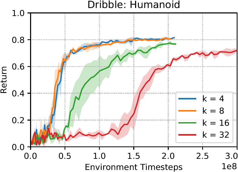
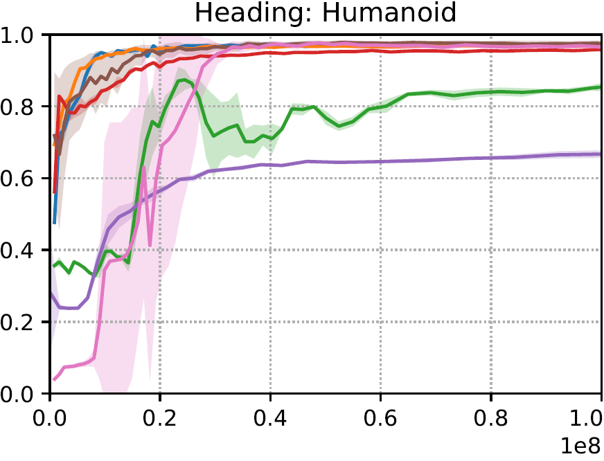
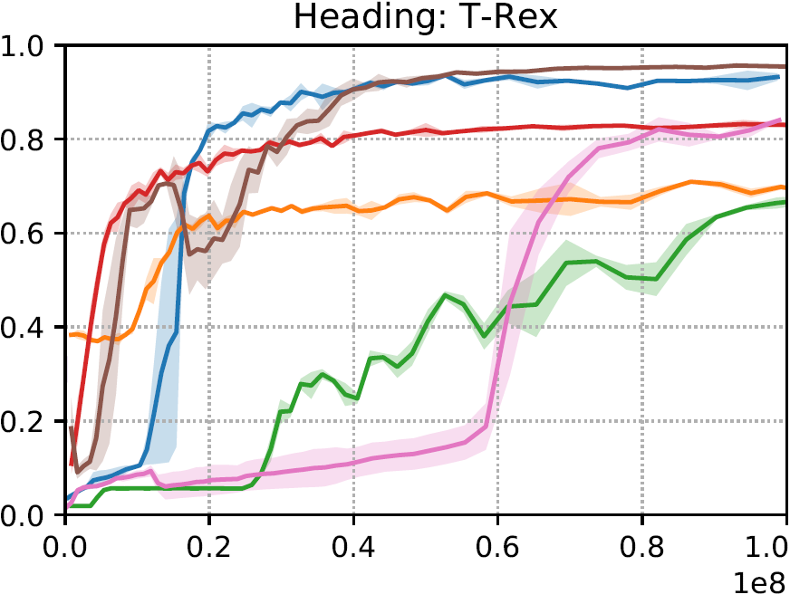
Supplementary curves count environment interactions, including the lower-frequency hierarchical controller fairly in physical timesteps. Four and eight MCP primitives perform similarly; increasing to sixteen or thirty-two slows learning in these tests. Thirty-two composition weights exceed the humanoid’s 28-dimensional action space, weakening the intended reduction in control dimensionality.
Refer to caption
Refer to caption
Refer to caption
Refer to caption
Refer to caption
Refer to caption
Refer to caption
Refer to caption
Refer to caption
Figure 8: Learning curves of the various models when applied to transfer tasks. MCP improves learning speed and performance on challenging tasks (e.g. carry and dribble), and is the only method that succeeds on the most difficult task (Dribble: T-Rex).
Environment Scratch Finetune Hierarchical Option-Critic MOE Latent Space MCP (Ours)
Heading: Biped 0.927±0.0320.927\pm 0.032 0.970±0.0020.970\pm 0.002 0.834±0.0010.834\pm 0.001 0.952±0.0120.952\pm 0.012 0.918±0.0020.918\pm 0.002 0.970±0.0010.970\pm 0.001 0.976±0.002\bf{0.976\pm 0.002}
Heading: Humanoid 0.965±0.0100.965\pm 0.010 0.975±0.008\bf{0.975\pm 0.008} 0.681±0.0060.681\pm 0.006 0.958±0.0010.958\pm 0.001 0.857±0.0180.857\pm 0.018 0.969±0.0020.969\pm 0.002 0.970±0.0030.970\pm 0.003
Heading: T-Rex 0.840±0.0030.840\pm 0.003 0.953±0.004\bf{0.953\pm 0.004} −- 0.830±0.0040.830\pm 0.004 0.672±0.0110.672\pm 0.011 0.686±0.0030.686\pm 0.003 0.932±0.0070.932\pm 0.007
Carry: Biped 0.027±0.0350.027\pm 0.035 0.324±0.0140.324\pm 0.014 0.001±0.0020.001\pm 0.002 0.346±0.0110.346\pm 0.011 0.013±0.0130.013\pm 0.013 0.456±0.0310.456\pm 0.031 0.575±0.032\bf{0.575\pm 0.032}
Dribble: Biped 0.072±0.0120.072\pm 0.012 0.651±0.0250.651\pm 0.025 0.546±0.0240.546\pm 0.024 0.046±0.0080.046\pm 0.008 0.073±0.0210.073\pm 0.021 0.768±0.0120.768\pm 0.012 0.782±0.008\bf{0.782\pm 0.008}
Dribble: Humanoid 0.076±0.0240.076\pm 0.024 0.598±0.0300.598\pm 0.030 0.198±0.0020.198\pm 0.002 0.058±0.0070.058\pm 0.007 0.043±0.0210.043\pm 0.021 0.751±0.0060.751\pm 0.006 0.805±0.006\bf{0.805\pm 0.006}
Dribble: T-Rex 0.065±0.0320.065\pm 0.032 0.074±0.0110.074\pm 0.011 −- 0.098±0.0130.098\pm 0.013 0.070±0.0170.070\pm 0.017 0.115±0.0130.115\pm 0.013 0.781±0.021\bf{0.781\pm 0.021}
Holdout: Ant 0.951±0.093\bf{0.951\pm 0.093} 0.885±0.0620.885\pm 0.062 −- −- −- 0.745±0.0600.745\pm 0.060 0.812±0.0300.812\pm 0.030
Table 2: Performance statistics of different models on transfer tasks.
Property Biped Humanoid T-Rex
Links 12 13 20
Total Mass (kg) 42 45 54.5
Height (m) 1.34 1.62 1.66
Degrees-of-Freedom 23 34 55
State Features 105 196 261
Action Parameters 17 28 49
Table 3: Properties of the characters.
Refer to caption
Table 4: Learning curves of MCP with different numbers of primitives kk.

8 Reference Motions

Biped and humanoid pretraining uses 230 seconds of motion-capture walking and turning. Retargeting to the biped removes unused upper-body joints. The T-Rex uses only eleven seconds of hand-authored walking and turning animation, showing reuse from a small but deliberately relevant repertoire.

9 Transfer Tasks

These sections specify goal state, randomization, and reward shaping for each transfer task.

Heading:

Heading changes by a uniform perturbation between −0.15 and 0.15 radians each step. Reward favors center-of-mass velocity of one meter per second along the requested direction.

Equation
rt=exp⁡(−4​(u^⋅vc​o​m−v^)2).r_{t}=\mathrm{exp}\left(-4\ \left(\hat{u}\cdot v_{com}-\hat{v}\right)^{2}\right).

Carry:

The five-kilogram box and destination are randomized up to ten meters apart. A virtual joint attaches the box after contact with a designated body link and detaches it at the destination. Reward combines approaching the box, staying near it, moving it toward the target, and reducing target distance, with weights 0.1/0.2/0.3/0.4. This is simplified carrying rather than learned physical grasping.

Equations
rt=wc​v​rtc​v+wc​p​rtc​p+wb​v​rtb​v+wb​p​rtb​p,r_{t}=w^{cv}r^{cv}_{t}+w^{cp}r^{cp}_{t}+w^{bv}r^{bv}_{t}+w^{bp}r^{bp}_{t},
rtc​v=exp⁡(−1.5​min​(0,ub⋅vc​o​m−v^)2)r^{cv}_{t}=\mathrm{exp}\left(-1.5\ \mathrm{min}\left(0,u_{b}\cdot v_{com}-\hat{v}\right)^{2}\right)
rtc​p=exp⁡(−0.25​‖xc​o​m−xb‖2).r^{cp}_{t}=\mathrm{exp}\left(-0.25\ ||x_{com}-x_{b}||^{2}\right).
rtb​v=exp⁡(−1​min​(0,ut​a​r⋅vb−v^)2)r^{bv}_{t}=\mathrm{exp}\left(-1\ \mathrm{min}\left(0,u_{tar}\cdot v_{b}-\hat{v}\right)^{2}\right)
rtb​p=exp⁡(−0.5​‖xb−xt​a​r‖2).r^{bp}_{t}=\mathrm{exp}\left(-0.5\ ||x_{b}-x_{tar}||^{2}\right).

Dribble:

Ball and goal locations are randomized up to ten meters apart. Reward balances approaching and remaining near the ball with advancing it toward the target, using weights 0.1/0.1/0.3/0.5. Unlike carrying, motion of the ball depends on contact dynamics without an attachment joint.

Equations
rt=wc​v​rtc​v+wc​p​rtc​p+wb​v​rtb​v+wb​p​rtb​p,r_{t}=w^{cv}r^{cv}_{t}+w^{cp}r^{cp}_{t}+w^{bv}r^{bv}_{t}+w^{bp}r^{bp}_{t},
rtc​v=exp⁡(−1.5​min​(0,ub⋅vc​o​m−v^)2)r^{cv}_{t}=\mathrm{exp}\left(-1.5\ \mathrm{min}\left(0,u_{b}\cdot v_{com}-\hat{v}\right)^{2}\right)
rtc​p=exp⁡(−0.5​‖xc​o​m−xb‖2).r^{cp}_{t}=\mathrm{exp}\left(-0.5\ ||x_{com}-x_{b}||^{2}\right).
rtb​v=exp⁡(−1​min​(0,ut​a​r⋅vb−v^)2)r^{bv}_{t}=\mathrm{exp}\left(-1\ \mathrm{min}\left(0,u_{tar}\cdot v_{b}-\hat{v}\right)^{2}\right)
rtb​p=exp⁡(−0.5​‖xb−xt​a​r‖2).r^{bp}_{t}=\mathrm{exp}\left(-0.5\ ||x_{b}-x_{tar}||^{2}\right).

Holdout:

The ant is pretrained on heading angles from zero to 3π/2, then transferred to the remaining quarter-circle. Reward adapts the usual locomotion objective to the requested direction while retaining health, control, and contact terms. This measures adaptation beyond the pretrained direction range.

Equations
rt=wforward​rtforward+whealthy​rthealthy+wcontrol​rtcontrol+wcontact​rtcontact,\displaystyle r_{t}=w^{\text{forward}}r_{t}^{\text{forward}}+w^{\text{healthy}}r_{t}^{\text{healthy}}+w^{\text{control}}r_{t}^{\text{control}}+w^{\text{contact}}r_{t}^{\text{contact}},
rtforward=u^⋅vc​o​m\displaystyle r_{t}^{\text{forward}}=\hat{u}\cdot v_{com}

10 Model Setup

Most models use PPO; option-critic follows its original updates. Discount factors are 0.95 during pretraining and 0.99 during transfer. Value fitting uses multi-step TD returns and policy updates use GAE.

10.1 mcp

MCP uses eight primitives and a value network with 1,024 and 512 hidden units. Table 5 specifies character-specific learning rates, batch size 4,096, minibatches 256, momentum 0.9, and PPO clipping 0.02.

Parameter Biped Humanoid T-Rex
kk Primitives 88 88 88
π\pi Stepsize (Pre-Train) 2×10−52\times 10^{-5} 1×10−51\times 10^{-5} 1×10−51\times 10^{-5}
π\pi Stepsize (Transfer) 5×10−55\times 10^{-5} 5×10−55\times 10^{-5} 5×10−55\times 10^{-5}
VV Stepsize 1×10⁻²¹\times 10^{-2} 1×10⁻²¹\times 10^{-2} 1×10⁻²¹\times 10^{-2}
Batch Size 40964096 40964096 40964096
Minibatch Size 256256 256256 256256
SGD Momentum 0.90.9 0.90.9 0.90.9
TD(λ\lambda) 0.950.95 0.950.95 0.950.95
GAE(λ\lambda) 0.950.95 0.950.95 0.950.95
PPO Clip Threshold 0.020.02 0.020.02 0.020.02

Table 5: MCP model hyperparamters.

10.2 Scratch

The scratch baseline learns a Gaussian action policy directly on each transfer task using 1,024- and 512-unit hidden layers, fixed diagonal covariance, and a matching value architecture. Table 6 preserves its tuned learning rates.

Parameter Biped Humanoid T-Rex
π\pi Stepsize 2.5×10−62.5\times 10^{-6} 2.5×10−62.5\times 10^{-6} 1×10−61\times 10^{-6}
VV Stepsize 1×10⁻²¹\times 10^{-2} 1×10⁻²¹\times 10^{-2} 1×10⁻²¹\times 10^{-2}
Batch Size 40964096 40964096 40964096
Minibatch Size 256256 256256 256256
SGD Momentum 0.90.9 0.90.9 0.90.9
TD(λ\lambda) 0.950.95 0.950.95 0.950.95
GAE(λ\lambda) 0.950.95 0.950.95 0.950.95
PPO Clip Threshold 0.020.02 0.020.02 0.020.02

Table 6: Scratch model hyperparamters.

10.3 Finetuning

The fine-tuning baseline first imitates a reference motion, then updates the same full policy on transfer tasks. Additional goal inputs are inserted without changing its initial behavior; its architecture otherwise matches scratch training.

Parameter Biped Humanoid T-Rex
π\pi Stepsize 2.5×10−62.5\times 10^{-6} 2.5×10−62.5\times 10^{-6} 1×10−61\times 10^{-6}
VV Stepsize 1×10⁻²¹\times 10^{-2} 1×10⁻²¹\times 10^{-2} 1×10⁻²¹\times 10^{-2}
Batch Size 40964096 40964096 40964096
Minibatch Size 256256 256256 256256
SGD Momentum 0.90.9 0.90.9 0.90.9
TD(λ\lambda) 0.950.95 0.950.95 0.950.95
GAE(λ\lambda) 0.950.95 0.950.95 0.950.95
PPO Clip Threshold 0.020.02 0.020.02 0.020.02

Table 7: Finetune model hyperparamters.

10.4 Hierarchical

The hierarchical baseline has seven separately trained walking or turning primitives. Frozen skills are selected once per approximately one-second gait cycle by a learned gate. This temporal selection frequency differs from the other controllers and is accounted for using environment-step comparisons.

Parameter Biped Humanoid
kk Primitives 77 77
π\pi Stepsize 1×10⁻³¹\times 10^{-3} 1×10⁻³¹\times 10^{-3}
VV Stepsize 1×10⁻²¹\times 10^{-2} 1×10⁻²¹\times 10^{-2}
Batch Size 40964096 40964096
Minibatch Size 256256 256256
SGD Momentum 0.90.9 0.90.9
TD(λ\lambda) 0.950.95 0.950.95
GAE(λ\lambda) 0.950.95 0.950.95
PPO Clip Threshold 0.020.02 0.020.02

Table 8: Hierarchical model hyperparamters.

10.5 Option-Critic

Option-critic learns eight options and termination functions during imitation. Both see state only, while the option-value function also sees goals. Transfer freezes options and terminations and learns new option values; joint fine-tuning was tried but produced degradation without clear gains.

Parameter Biped Humanoid T-Rex
kk Options 88 88 88
π\pi Stepsize 2.5×10−62.5\times 10^{-6} 2.5×10−62.5\times 10^{-6} 1×10−61\times 10^{-6}
βω\beta_{\omega} Stepsize 2.5×10−62.5\times 10^{-6} 2.5×10−62.5\times 10^{-6} 1×10−61\times 10^{-6}
QΩQ_{\Omega} Stepsize 1×10⁻²¹\times 10^{-2} 1×10⁻²¹\times 10^{-2} 1×10⁻²¹\times 10^{-2}
Batch Size 256256 256256 256256
SGD Momentum 0.90.9 0.90.9 0.90.9
ξ\xi Termination Cost 0.010.01 0.010.01 0.010.01

Table 9: Option-critic model hyperparamters.

10.6 Mixture-of-Experts

The additive MOE comparison also trains eight state-conditioned primitives and a goal-aware gate. It freezes primitives for transfer but samples only one primitive at each step. This isolates an important difference from simultaneous product composition.

Parameter Biped Humanoid T-Rex
kk Primitives 88 88 88
π\pi Stepsize 1×10−51\times 10^{-5} 5×10−65\times 10^{-6} 2×10−62\times 10^{-6}
VV Stepsize 1×10⁻²¹\times 10^{-2} 1×10⁻²¹\times 10^{-2} 1×10⁻²¹\times 10^{-2}
Batch Size 40964096 40964096 40964096
Minibatch Size 256256 256256 256256
SGD Momentum 0.90.9 0.90.9 0.90.9
TD(λ\lambda) 0.950.95 0.950.95 0.950.95
GAE(λ\lambda) 0.950.95 0.950.95 0.950.95
PPO Clip Threshold 0.020.02 0.020.02 0.020.02

Table 10: Mixture-of-experts model hyperparamters.

10.7 Latent Space

The latent baseline uses an eight-dimensional Gaussian code with KL regularization toward a standard Gaussian. A pretrained decoder maps state and code into actions; transfer freezes that decoder and learns a new state-and-goal encoder. Its complete architecture and hyperparameters remain in Table 11.

Equation 5
arg​maxπ,q𝔼τ∼pπ,q​(τ)[∑t=0Tγtrt]+β𝔼gt∼p⁡(gt)[DK​L[q(wt|gt)||p0(wt)]]\mathop{\mathrm{arg\ max}}_{\pi,q}\quad\mathbb{E}_{\tau\sim p_{\pi,q}(\tau)}\left[\sum_{t=0}^{T}\gamma^{t}r_{t}\right]+\beta\ \mathbb{E}_{g_{t}\sim p(g_{t})}\left[\mathrm{D}_{KL}\left[q(w_{t}|g_{t})\middle||p_{0}(w_{t})\right]\right] (5)
Parameter Biped Humanoid T-Rex
ww Latent Size 88 88 88
π\pi Stepsize (Pre-Train) 5×10−65\times 10^{-6} 2.5×10−62.5\times 10^{-6} 1×10−61\times 10^{-6}
π\pi Stepsize (Transfer) 5×10−55\times 10^{-5} 5×10−55\times 10^{-5} 5×10−55\times 10^{-5}
VV Stepsize 1×10⁻²¹\times 10^{-2} 1×10⁻²¹\times 10^{-2} 1×10⁻²¹\times 10^{-2}
Batch Size 40964096 40964096 40964096
Minibatch Size 256256 256256 256256
SGD Momentum 0.90.9 0.90.9 0.90.9
TD(λ\lambda) 0.950.95 0.950.95 0.950.95
GAE(λ\lambda) 0.950.95 0.950.95 0.950.95
PPO Clip Threshold 0.020.02 0.020.02 0.020.02
β\beta KL Regularizer 1×10−41\times 10^{-4} 1×10−41\times 10^{-4} 1×10−41\times 10^{-4}

Table 11: Latent space model hyperparamters.
Concept demonstration

Open image ↗