Overview
The supplementary material provides optimization and curriculum details, task configurations and data generation, a visual-input extension, a constructive expressiveness argument, sample symbolic blocks-world rules, and a minimal TensorFlow implementation. These appendices qualify how to interpret the main paper’s generalization results.
At a glance
Neural Logic Machines learn relational computations through shared neural transformations over object tuples, with explicit operations for permutation and quantification. The architecture can transfer a learned computation to larger object sets because its parameters do not depend on the number of objects. Selected trained models achieve perfect accuracy on the reported symbolic tests, but optimization sometimes fails and the experiments do not prove correctness on every possible larger instance.
1 Introduction
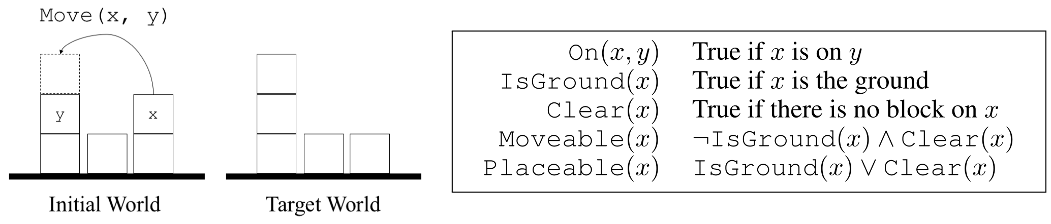
The motivating blocks-world task requires identifying legal moves and rearranging blocks into a target configuration. It combines several challenges: transferring across object counts, representing relations involving more than two objects, composing many intermediate predicates, and learning without task-specific rule templates. NLM addresses these with tensorized predicates and shared neural modules. The actual experiments still supply substantial structure through symbolic inputs, comparison relations, chosen depth/arity, curriculum, and—in blocks world—auxiliary action-validity supervision.
2 Neural Logic Machines (NLM)
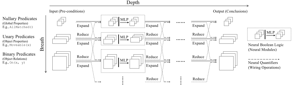
Under the closed-world assumption, known predicates are grounded over a finite set of objects. NLM layers transform these premise tensors into intermediate and output predicates. Shared Boolean transformations approximate logical connectives, while fixed wiring aligns arities and performs quantification. The learned rules are implicit neural weights; producing a human-readable symbolic rule set is left for future work.
2.1 Logic Predicates as Tensors
A predicate of arity r assigns a value to each ordered tuple of distinct objects. The representation excludes repeated arguments; their values can instead be represented by suitable lower-arity predicates. Channels collect multiple predicates of the same arity, and a nullary group represents global properties. Values lie between zero and one and are interpreted as soft truth values, without a separate calibration guarantee. Maximum arity B is called breadth. Arguments are objects or variables, without function symbols, following the finite Datalog-style setting.
2.2 Logic Rules as Neural Operators
For each tuple, the model gathers every permutation of its arguments and applies the same multilayer perceptron followed by sigmoid. Parameter sharing makes the rule lifted across object identities. The r! permutation factor is a real cost even though it is treated as constant in fixed-breadth complexity expressions.
Expansion adds a new argument by replicating a lower-arity predicate. Reduction removes an argument with maximum or minimum, implementing existential or universal quantification on Boolean inputs. Concatenating both reductions doubles the channel count. The original ValidMove and Moveable examples show how predicates with different argument sets are aligned before combining them; all example rules and equations remain below. With soft truth values, max/min are the architecture’s chosen differentiable logical relaxation.
Equations 1–4
| (1) |
| (2) |
| (Expansion) | (3) |

| (Reduction) | (4) |

2.3 Neural Logic Machines
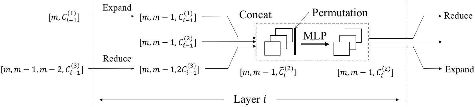
At each layer and arity, expansion of the preceding lower-arity group, the same-arity group, and reduction of the higher-arity group are concatenated. All argument permutations are then passed through a shared neural transformation. Boundary groups omit nonexistent neighbors. Figure 3 shows the binary case, which combines unary, binary, and ternary inputs. Layers compute in parallel from the previous layer. The expressiveness discussion assumes sufficient depth, breadth, channels, and neural capacity and excludes cyclic predicate dependencies in its constructive proof.
Equations 5–6
| (5) |
| (6) |
2.4 Expressiveness and Computational Complexity
Depth bounds deduction steps; breadth bounds tuple arity; channel count bounds intermediate predicates; neural width and depth bound the Boolean transformations. For fixed small breadth, the stated forward/backward cost is O(mᴮDC²) with O(DC²) parameters. Constants hide the factorial permutation dependence on breadth, and tensors still grow rapidly with the object count m. Independence of parameter count from m therefore does not mean constant computation or memory when transferring to larger instances.
3 Experiments
Supervised family and graph tasks train on all target object or pair labels. Sequential blocks-world, sorting, and path tasks use reinforcement learning with an exam-guided curriculum. The appendix reports both test performance and the probability of successfully graduating from training. Perfect accuracy of a selected successful model should be distinguished from reliable success across random initializations.
3.1 Baselines
The principal comparisons are Memory Networks and differentiable inductive logic programming. Memory Networks encode object identifiers and predicate values as memory entries, then answer object or pair queries through recurrent lookup. The differentiable ILP baseline consumes grounded predicates. Additional DNC and graph-network numbers come from related setups and should not be treated as fully controlled identical-task comparisons.
3.2 Family tree reasoning
Models learn family relations from randomly generated twenty-person families and are evaluated at twenty and one hundred people. Inputs are son, daughter, father, and mother relations; outputs include parent existence, sisters, grandparents, uncles, and maternal great uncles. NLM and differentiable ILP reach 100% in the table, while Memory Networks often lose accuracy at the larger size. Memory Network entries report micro and macro accuracy. The separately cited DNC result asks for identification of a maternal great uncle rather than binary classification of every pair.
| Family Tree | MemNN | ILP | NLM (Ours) | |||
|---|---|---|---|---|---|---|
| HasFather | 99.9% / 99.9% | 59.8% / 65.2% | 100% | 100% | 100% | 100% |
| HasSister | 86.3% / 85.5% | 59.8% / 66.4% | 100% | 100% | 100% | 100% |
| IsGrandparent | 96.5% / 84.7% | 97.7% / 63.7% | 100% | 100% | 100% | 100% |
| IsUncle | 96.3% / 85.8% | 96.0% / 64.0% | 100% | 100% | 100% | 100% |
| IsMGUncle | 99.7% / 98.4% | 98.4% / 81.7% | 100% | 100% | 100% | 100% |
| Graph | MemNN | ILP | NLM (Ours) | |||
| AdjacentToRed | 95.2% / 94.6% | 93.1% / 91.9% | 100% | 100% | 100% | 100% |
| -Connectivity | 92.3% / 90.5% | 81.3% / 88.0% | 100% | 100% | 100% | 100% |
| -Connectivity | 67.6% / 58.8% | 43.9% / 67.9% | 100% | 100% | 100% | 100% |
| -OutDegree | 99.8% / 99.7% | 78.6% / 81.2% | 100% | 100% | 100% | 100% |
| -OutDegree | 81.4% / 61.8% | 96.7% / 87.7% | N/A | N/A | 100% | 100% |
3.3 General graph reasoning
Graphs supply adjacency and node colors. Tasks predict adjacency to a red node, connectivity within four or six edges, and exact out-degree one or two. Training uses ten nodes and testing uses ten or fifty. NLM reports 100% on these tests; differentiable ILP cannot fit the stated two-out-degree construction within its memory constraint. This is an implementation/scalability limitation of that comparison, not proof that symbolic logic cannot express the task. Exact two-out-degree uses breadth four in the appendix configuration.
3.4 Blocks World
The operating and target worlds contain corresponding blocks and a ground object. Inputs compare world identity, object identity, and coordinates across object pairs. Actions move one block onto another block or the ground; invalid actions leave the state unchanged. The reported NLM completes all sampled ten- and fifty-block cases, averaging twelve and eighty-four moves, while Memory Networks complete none within the stated limit. Appendix B.5 supplies an important implementation qualification: the action head manually joins current and target object representations by identity and uses an additional supervised validity/effect-prediction loss.
| Task | MemNN | NLM (Ours) | ||
|---|---|---|---|---|
| BlocksWorld | 0% / N/A | 0% / N/A | 100% / 12 | 100% / 84 |
| Sorting | 100% / 22 | 90% / 986.6 | 100% / 8 | 100% / 45 |
| Path | 45% / 13.3 | 12% / 42.7 | 100% / 4 | 100% / 4 |
3.5 General algorithms
Sorting. The model receives comparisons of indices and values for every pair and chooses swaps. Thus pairwise comparison work is already supplied as input. NLM solves the reported ten- and fifty-element tests in an average of eight and forty-five swaps. Different learned policies resemble familiar sorting procedures, but no extracted symbolic program or universal correctness proof is provided.
Path finding. The policy moves the current node toward a marked target using adjacency and node markers. Training source–target distance is at most five; testing distance is four even when the graph grows to fifty nodes. Perfect four-step test paths demonstrate transfer across graph size under this bounded-distance setup, not extrapolation to arbitrarily long paths. The project page includes examples of learned behavior.
4 Related works and discussions
NLM replaces explicit search over many candidate symbolic rules with learned tuple transformations. Its comparison with message-passing graph networks emphasizes higher-arity intermediate relationships, while its comparison with ILP emphasizes compositional capacity and optimization over weights. These advantages come with all-tuple tensor cost and reduced direct interpretability.
The discussion places NLM alongside relational reinforcement learning, generalized planning, neural program induction, and differentiable perception. The authors explicitly leave scaling to very large entity sets unresolved; the demonstrated finite object domains differ from large knowledge-base completion settings.
5 Conclusions and Discussions
The architecture offers a useful relational inductive bias for learning computations that transfer across object counts. Remaining issues include selecting depth adaptively, handling general real-valued inputs, simplifying difficult optimization, extracting readable rules, and scaling tensors to large domains. Its proof covers an acyclic finite rule family with enough capacity; empirical success after curriculum training does not remove these restrictions.
Acknowledgements
The authors acknowledge Rishabh Singh, Thomas Walsh, the area chair, and reviewers for feedback.
Appendix A Training Method and Curriculum Learning
The appendix specifies the optimization losses, exploration controls, reward shaping, and curriculum that enable the sequential tasks. These details are part of the experimental method rather than incidental implementation choices.
A.1 Training method
Both architectures use Adam at learning rate 0.005. Supervised batches contain four instances. Reinforcement learning uses one episode per update with REINFORCE and an entropy bonus, discount 0.99, terminal success reward one, and a −0.01 penalty per move. Thus the decision tasks have sparse success feedback but also step-cost shaping. Table 3 gives task-dependent exploration weights, episode budgets, and limits: sorting trains on sizes four through ten, path on three through twelve, and blocks world on two through twelve.
Equation
| Task | Range |
|
Epochs |
|
| ||||||||
|---|---|---|---|---|---|---|---|---|---|---|---|---|---|
| Sorting | [4, 10] | 0.01 | 0.5 | 5 | 200 | 200 | |||||||
| Path | [3, 12] | 0.1 | 0.5 | 40 | 600 | 3000 | |||||||
| Blocks World | [2, 12] | 0.2 | 0.6 | 50 | 1000 | 3000 |
A.2 Curriculum learning guided by exams and fails
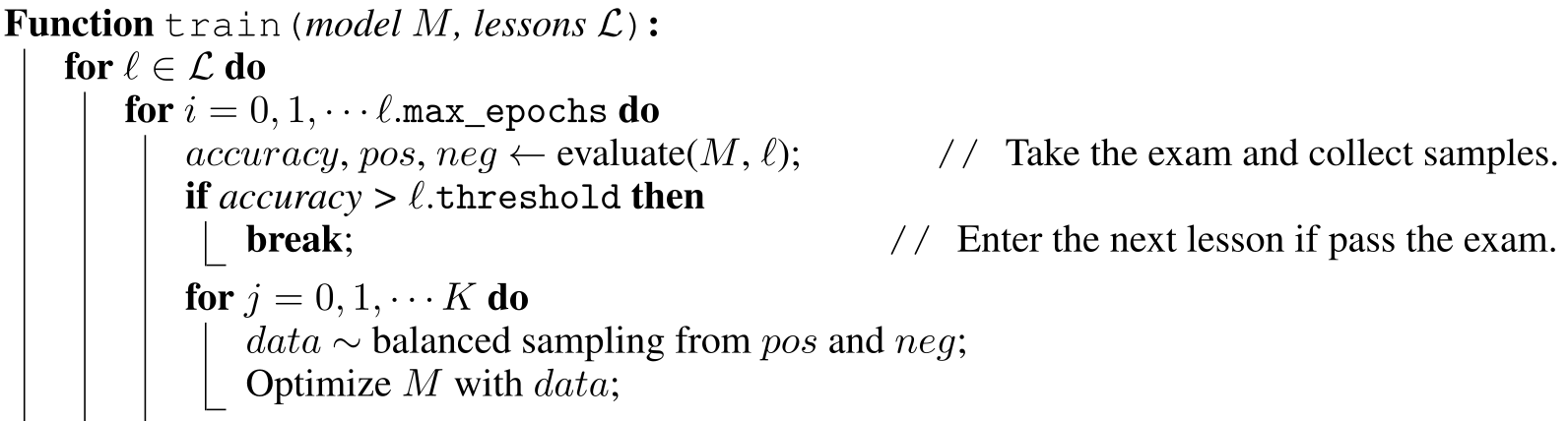
Lessons increase the object count. Exams sample the three most recent lesson sizes; success and failure instances populate separate pools, and training samples the positive pool with task-dependent probability Ω. The final stated graduation target is 100% success, with earlier thresholds relaxed by half a percentage point per lesson. Algorithm 1 retains the original strict-greater-than comparison, which is inconsistent with literally exceeding a final 100% threshold; the prose describes passing at 100%. The curriculum and failure-balanced sampling are substantial training support, and a run can fail to graduate.
Appendix B Implementation details and hyper-parameters
Implementation details cover residual input access, per-task model capacity, baseline settings, synthetic distributions, the blocks-world action head, and finite-sample accuracy claims. Table 4 is essential for distinguishing representational generalization from the difficulty of obtaining a successful model.
B.1 Residual connection.
Residual links concatenate the original predicate channels with the newly inferred channels separately for each arity. They preserve access to base facts through deeper computations, rather than performing an additive residual update.
B.2 Hyper-parameters for NLM
All reported NLM Boolean modules use no hidden layer, and intermediate groups have eight predicate channels. Table 4 varies depth from three to eight and breadth from two to four. Graduation means a task-specific supervised loss threshold, usually 10⁻⁶, or a perfect final curriculum exam. Across ten seeds, graduation is only 20% for maternal great uncle, 40% for blocks world, and 60% for path and six-connectivity. Increasing family training size to thirty raises maternal-great-uncle graduation to 50%. These rates qualify the headline perfect-test results.
| Tasks | Depth | Breath | Res. | Grad. | Num. Examples/Episodes | |
|---|---|---|---|---|---|---|
| Family Tree | HasFather | 4 | 3 | × | 100% | 50,000 examples |
| HasSister | 4 | 3 | × | 100% | 50,000 examples | |
| IsGrandparent | 4 | 3 | × | 100% | 100,000 examples | |
| IsUncle | 4 | 3 | × | 90% | 100,000 examples | |
| IsMGUncle | 4 | 3 | × | 20% | 200,000 examples | |
| General Graph | AdajacentToRed | 4 | 3 | × | 90% | 100,000 examples |
| -Connectivity | 4 | 3 | × | 100% | 50,000 examples | |
| -Connectivity | 8 | 3 | ✓ | 60% | 50,000 examples | |
| -OutDegree | 4 | 3 | × | 100% | 50,000 examples | |
| -OutDegree | 5 | 4 | ✓ | 100% | 100,000 examples | |
| General Algorithm | Sorting | 3 | 2 | ✓ | 100% | 1,000 episodes |
| Path | 5 | 3 | ✓ | 60% | 24,000 episodes | |
| BlocksWorld | 7 | 2 | ✓ | 40% | 50,000 episodes | |
B.3 Hyper-parameters for MemNN
Memory Networks receive the same stated iteration or episode budgets. Key and value dimensions are sixteen and thirty-two, the recurrent state has sixty-four units, and lookup uses four queries except for one in sorting. The authors report a hyperparameter search with little improvement, but the comparison is still tied to this encoding and architecture configuration.
B.4 Data generation
Family trees are generated by a timeline of new people, sampled genders, parents, and marriages, then permuted. Graphs place nodes in a unit square, sample degrees, and connect nearest neighbors, optionally treating edges as undirected. Sorting samples permutations. Blocks world adds each block onto a randomly selected available support and then shuffles identities. Test conclusions apply to these synthetic generators; random sampling does not enumerate every graph or arrangement.
B.5 Blocks World
Blocks-world training adds a cross-entropy objective predicting action validity or effects with weight 0.1. The implementation joins current and target representations for the same object, forms pair features, and applies a fully connected softmax action head. This is more specialized than directly using final pair predicates. Consequently, describing the demonstrated policy as learned solely from a terminal success signal would omit both auxiliary supervision and the supplied correspondence structure.
B.6 Accuracy discussion
Reported task accuracies use one thousand randomly generated test cases. One specific trained blocks-world model is additionally tested on one hundred thousand cases without a failure; the authors give a Chernoff-based 99.7% confidence statement that accuracy is at least 99.98%. This is a sampling statement for that model and test distribution, not a proof from recovered symbolic rules, a guarantee on all larger inputs, or a statement that every training run succeeds.
Appendix C Neural Logic Machines (NLM) extensions
The visual-input extension replaces graph-node colors with MNIST digits and asks whether a node is adjacent to a zero. A jointly trained LeNet produces ten sigmoid features per node for NLM reasoning. Training uses one hundred thousand ten-node examples and the standard MNIST training split; evaluation on one thousand fifty-node examples reports 99.4%. This controlled digit-recognition extension shows end-to-end differentiability, while leaving broader noisy perception and arbitrary continuous inputs open.
Appendix D Realization of Horn Clause
The constructive proof assumes enough layers, breadth, and channels. For one definite clause, it expands body predicates to a common variable set, uses permutations and a neural Boolean transformation to combine them, reduces body-only variables by existential quantification, and expands any head-only variables. Facts are tensor entries. Multiple rules with one head are combined by disjunction.
For an acyclic set of rule dependencies, topological ordering lets these constructions be stacked into forward chaining. Cyclic references and unrestricted recursion are explicitly deferred. The argument establishes representability of this rule family under sufficient capacity; it does not prove gradient descent learns the intended rule or that arbitrary finite sigmoid weights produce exact Boolean truth values without approximation.
Equations
Appendix E Sample Blocks World Rules
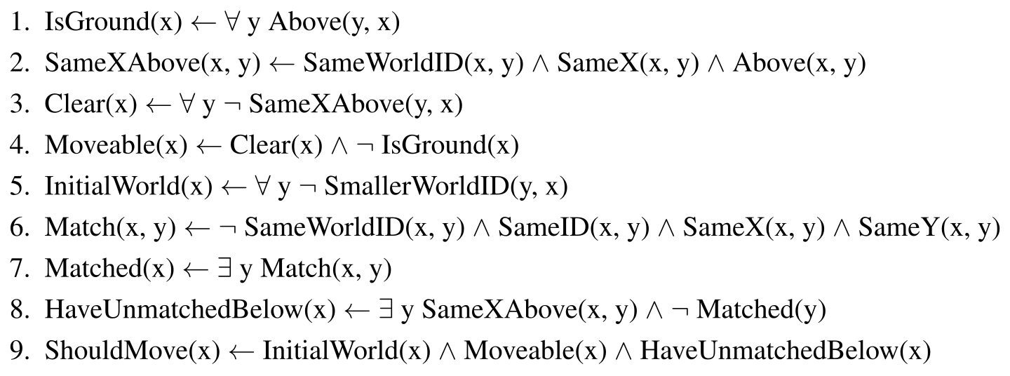
The hand-written example illustrates the complexity of deciding whether a block ought to move. It is an explanatory rule set supplied by the authors, not a rule program extracted from a trained network. Choosing a destination still requires additional logic.
Input Relations.
The nine helper rules derive ground, vertical same-world relations, clear and moveable blocks, initial-world membership, correspondence matches, unmatched blocks below, and finally ShouldMove. All nine rules and the original expanded expression are retained. They illustrate how quantification and intermediate predicates compose from pairwise comparisons. The example is only part of a complete policy, and the actual training procedure also includes the auxiliary objective documented in Appendix B.5.
Equations

Appendix F Implement NLM in TensorFlow
The original fifty-nine-line TensorFlow listing implements one breadth-three layer: broadcasting for expansion, masked max/min reductions that exclude repeated-object tuples, all argument permutations, shared dense sigmoid transformations, and optional concatenated residual inputs. The exact embedded source text and indentation are retained. It is historical illustrative code, not a complete training system; its interfaces and the spelling of the exported function are left as printed.
from itertools import permutations
import tensorflow as tf
from tensorflow.layers import dense

def expand(input, M):
  """Expands input at its second last dimension (e.g., [B, ..., Ni, Nj] to [B, ..., Ni, M, Nj]) by replicating tensors."""
  ndims = input.get_shape().ndims + 1
  multiples = [M if i == ndims - 2 else 1 for i in range(ndims)]
  return tf.tile(tf.expand_dims(input, -2), multiples)

def reduce(input, M):
  """Reduces max and min at the second last dimension, except for diagonal elements."""
  mask = _reduce_mask(input, M)[tf.newaxis, ..., tf.newaxis]
  return tf.concat([
    tf.reduce_max(input * mask, -2),
    tf.reduce_min(input * mask + (1 - mask), -2)
  ], -1)

def neural_logic(input, hidden_dim):
  """An MLP layer applied on permutations of the input."""
  return dense(_input_permutations(input), hidden_dim, activation=tf.sigmoid)

def neural_logic_layer_breath3(input0, input1, input2, input3, M, hidden_dim, residual):
  """A neural logic layer with breath 3.
  Args:
    input0: float Tensor of shape [B, hidden_dim], nullary predicates.
    input1: float Tensor of shape [B, M, hidden_dim], unary predicates.
    input2: float Tensor of shape [B, M, M, hidden_dim], binary predicates.
    input3: float Tensor of shape [B, M, M, M, hidden_dim], tenary predicates.
    M: int, number of objects.
    hidden_dim: int, hidden dimension.
    residual: boolean, use the residual link or not.
  Returns:
    4 float Tensors, output nullary, unary, binary tenary predicates respectively.
  """
  agg0 = tf.concat([input0, reduce(input1, M)], -1)
  agg1 = tf.concat([input1, expand(input0, M), reduce(input2, M)], -1)
  agg2 = tf.concat([input2, expand(input1, M), reduce(input3, M)], -1)
  agg3 = tf.concat([input3, expand(input2, M)], -1)
  outputs = [neural_logic(x, hidden_dim) for x in [agg0, agg1, agg2, agg3]]
  if residual:
    outputs = [tf.concat([x, y], -1) for x, y in zip(outputs, [input0, input1, input2, input3])]
  return outputs

def _reduce_mask(input, M):
  dimension = input.get_shape().ndims - 2
  base = 1.0 - tf.eye(M)
  if dimension < 2: return tf.constant(1.0)  # Identity.
  elif dimension == 2: return base # Diagonal excluded.
  elif dimension == 3: return tf.expand_dims(base, 2) * tf.expand_dims(base, 1) * tf.expand_dims(base, 0)  # Mask out all tuples (x, y, z) that x == y or y == z or z == x.
  else: raise NotImplementedError()

def _input_permutations(input):
  dimension = input.get_shape().ndims - 2
  if dimension < 2: return input
  else: return tf.concat([
    tf.transpose(input, [0] + list(perm) + [1 + dimension])
    for perm in permutations(range(1, 1 + dimension))
  ], -1)