At a glance
Intuition. Treat a layer’s weight matrix as a device that stretches signals differently in different directions. Its spectrum summarizes those stretching strengths, much like a histogram summarizes a large dataset. Comparing that histogram with an ideal random matrix can reveal structure worth investigating.
Reading the math. If a diagonal W stretches two axes by 3 and 1, WᵀW has eigenvalues 9 and 1: squared singular values. The empirical spectral density is simply their histogram across a layer. A heavy tail means large eigenvalues remain relatively common across scales. This can reveal correlations, but does not identify what the network knows or guarantee good test performance.
The paper studies empirical eigenvalue distributions of trained neural-network weight matrices using random matrix theory. Small or older models often resemble a Marchenko–Pastur bulk with a few separated eigenvalues; several larger pretrained models instead show broad, approximately power-law spectra. The authors interpret these patterns as forms of implicit self-regularization and organize them into five main regimes plus a rank-collapse regime. A MiniAlexNet batch-size sweep connects spectral changes with measured train/test accuracy. These are weight-spectrum diagnostics and a proposed phenomenological explanation, not a generalization bound or a proof that heavy tails cause better performance.
1 Introduction
The motivating question is why overparameterized networks can generalize without an obvious explicit complexity penalty. The authors propose inspecting weight matrices directly, complementing analyses of optimization, norms, and capacity. Random matrix theory supplies a reference for largely uncorrelated weights and for departures from that reference. The analysis concerns the eigenvalues of weight Gram matrices, not Hessians or the network’s complete input–output function. A layer spectrum alone cannot identify the training process, data distribution, or generalization error. The paper’s broad criticism of conventional capacity theory is motivation for its alternative diagnostic, rather than a demonstration that those theories are invalid.
Main Empirical Results.
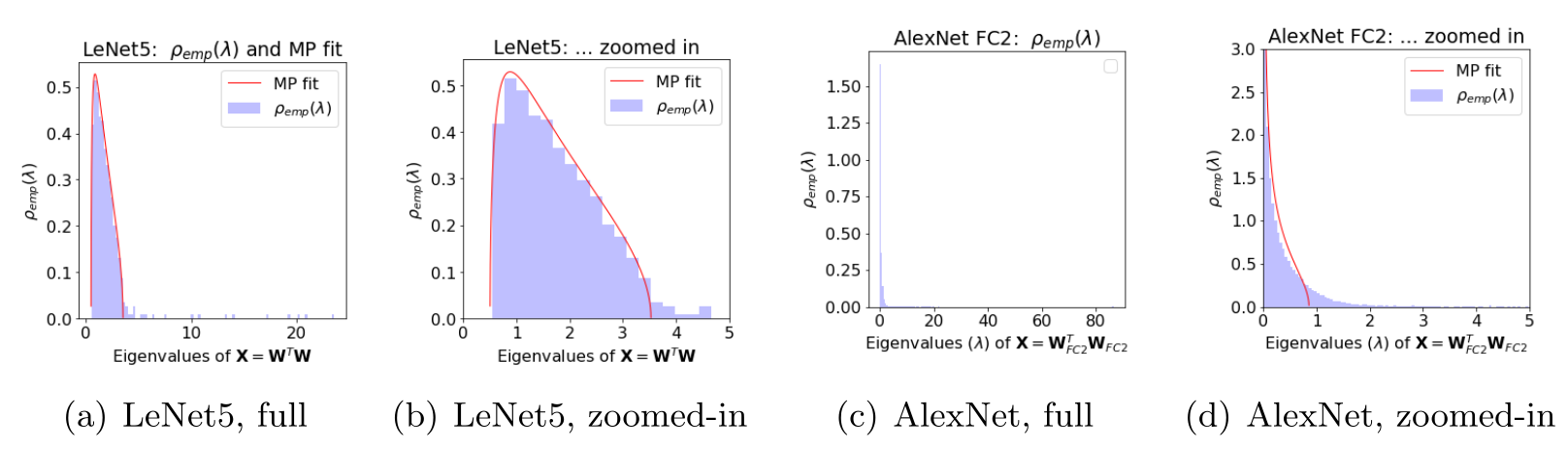
The empirical contrast is between a Marchenko–Pastur-like bulk with outlying eigenvalues in a small LeNet5 model and much heavier spectral tails in selected AlexNet and Inception layers. The former is interpreted as a noisy matrix plus relatively low-rank learned structure; the latter as correlations spanning many scales. The authors use “self-regularization” for structure emerging during ordinary training, even without an explicit penalty. Their selected model comparisons do not isolate architecture, data, size, and optimization as separate causes.
Main Theoretical Results.
The proposed model writes a weight matrix as a random component plus learned structure. Standard and spiked covariance ensembles motivate weakly correlated or low-rank cases, while heavy-tailed random ensembles act as surrogates for more strongly correlated learned matrices. This analogy does not require the actual learned entries to be independent or heavy-tailed. The resulting phase taxonomy mixes mathematical results for specified random ensembles with empirical fits and conjectural interpretations of neural-network weights. Those levels of evidence should remain distinct.
Evaluating the Theory.
The paper tests its interpretation by varying batch size in a small model and comparing spectra, rank-like statistics, and classification accuracy. The later sweep illustrates the five main regimes; rank collapse is also presented as a possible over-regularized regime. Although the introduction and Table 2 claim that all “5+1” phases are exhibited, the displayed batch-size sequence does not establish a separate rank-collapse experiment. The preserved figures allow that scope to be assessed directly.
2 Basic Random Matrix Theory (RMT)
The reference matrix has N rows and M columns, with N≥M and aspect ratio Q=N/M. Its M Gram-matrix eigenvalues define an empirical spectral distribution. Matrix normalization, finite size, and assumptions about independence and moments matter when comparing this distribution with an asymptotic law.
2.1 Marchenko-Pastur (MP) theory for rectangular matrices
For independent, centered, sufficiently regular entries, the Marchenko–Pastur law describes the limiting bulk of a normalized sample covariance matrix. Its support depends on the aspect ratio and variance; under stronger conditions, edge fluctuations have Tracy–Widom behavior. A fitted bulk edge can therefore serve as a reference for separated spectral mass, but a histogram fit alone does not verify the random-ensemble assumptions or edge statistics [Johnstone, 2001].
The source’s normalization convention needs care. It writes X=WᵀW while giving the usual support σ²(1±1/√Q)². If σ² is the variance of unscaled entries, that support applies to WᵀW/N; the unnormalized matrix acquires a factor of N. The displayed formula is consistent only if the weight or fitted-variance convention absorbs that normalization. The original equations are retained, rather than silently assigning a different meaning to σ.
Equations 1
| (1) |
2.2 Heavy-Tailed extensions of MP theory
The heavy-tail model defines an entry density proportional to |x|⁻⁽¹⁺μ⁾, so μ is the corresponding tail-probability exponent. Table 1 separates μ>4, 2<μ<4, and 0<μ<2, and explicitly labels some finite-size relations as phenomenological or conjectural. Heavy tails can produce extreme eigenvalues far beyond a conventional bulk edge; in the infinite-variance regime, the global spectral scaling itself changes. Finite-size fitting can obscure these distinctions.
A qualification is needed for the table’s global power-law description when 2<μ<4. Under the usual independent, centered, finite-variance assumptions, the normalized global empirical distribution can still converge to Marchenko–Pastur while extreme eigenvalues have heavy-tail behavior. A heavy far tail therefore does not by itself imply a globally power-law limiting density. This bulk-versus-extremes distinction is stated explicitly in the review by Davis, Heiny, Mikosch, and Xie. Likewise, N⁻²ᐟ³-type edge scaling describes appropriately centered fluctuations, rather than the location of the whole support edge.
For learned weights, the authors use these random ensembles as effective descriptions of correlations. They fit finite empirical spectra with the Clauset–Shalizi–Newman approach and compare power laws against alternatives including truncated power laws, exponentials, stretched exponentials, and lognormal distributions [Clauset et al., 2009]. A fitted spectral exponent is not a unique measurement of the entry-tail exponent or a proof of a particular correlation mechanism. The original formulas and table remain available with these assumptions in view.
|
Generative Model
w/ elements from Universality class |
Finite-
Global shape |
Limiting
Global shape |
Bulk edge
Local stats |
(far) Tail
Local stats | |
| Basic MP | Gaussian |
MP, i.e.,
Eqn. (1) |
MP | TW | No tail. |
|
Spiked-
Covariance |
Gaussian,
+ low-rank perturbations |
MP +
Gaussian spikes |
MP | TW | Gaussian |
|
Heavy tail,
|
(Weakly)
Heavy-Tailed |
MP +
PL tail |
MP | Heavy-Tailed∗ | Heavy-Tailed∗ |
|
Heavy tail,
|
(Moderately)
Heavy-Tailed (or “fat tailed”) |
PL∗∗
|
PL
|
No edge. | Frechet |
|
Heavy tail,
|
(Very)
Heavy-Tailed |
PL∗∗
|
PL
|
No edge. | Frechet |
Equation 2
| (2) |
3 Empirical Results: ESDs for Existing, Pretrained DNNs
A Keras LeNet5 model trained on MNIST reaches about 100% training and 99.25% test accuracy. Its 2,450×500 fully connected matrix shows a bulk below roughly 3.5, additional mass near 3.5–5, and separated eigenvalues extending toward 25. The authors interpret the bulk as noise-like and the separated modes as learned structure, analogous to a spiked covariance model or traditional regularization. This is a spectral interpretation, not a direct identification of signal and noise from labels.
For the examined 4,096×1,000 AlexNet layer, a Marchenko–Pastur fit is poor and the reported power-law exponent is about 2.25. Selected VGG, ResNet, and Inception layers also motivate a heavier-tailed description, with reported exponents often around 1.5–3.5, but not every layer or architecture fits identically. Several additional model results are described without full plots. The paper cautions that different fitting ranges and finite-size effects complicate comparisons. Figure 1 preserves the full four-panel contrast between the two representative layers.
4 5+1 Phases of Regularized Training
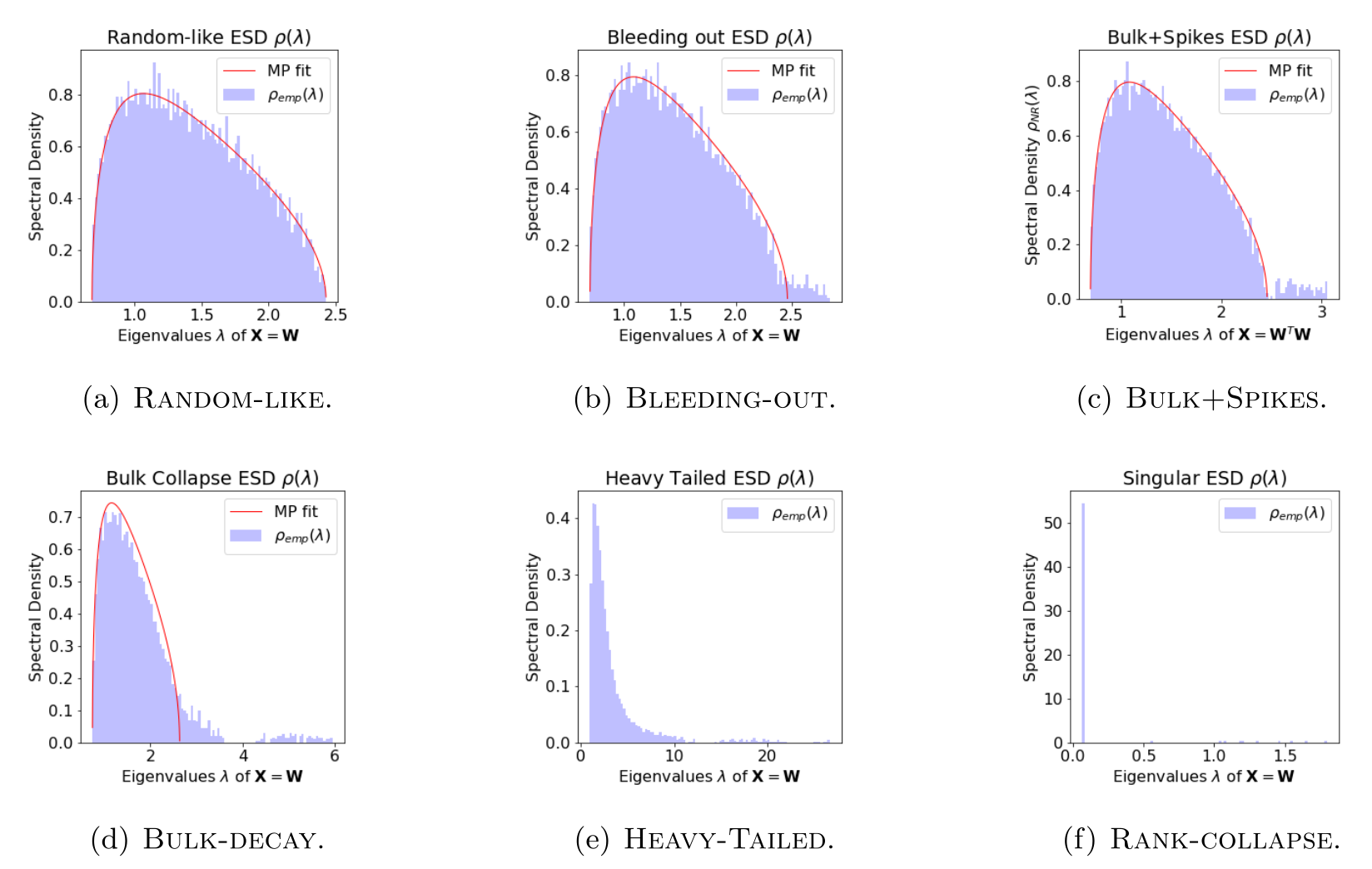
The proposed decomposition W≈W_rand+Δ_sig organizes six operational patterns. Random-like spectra admit a conventional bulk fit. Bleeding-out spectra develop excess mass near its upper edge. Bulk+Spikes retains a bulk with separated large eigenvalues. Bulk-decay weakens the clear bulk/spike separation. Heavy-Tailed spectra are better described by a broad heavy-tailed fit. Rank-collapse adds substantial mass at zero and represents severe rank deficiency or over-regularization. Table 2 and Figure 2 retain every regime and its stated interpretation.
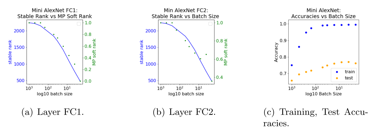
Spiked random-matrix results motivate some transition and edge-statistic language, but they do not establish that a trained network follows that ensemble or traverses these regimes in a universal order. Correlation strength is an interpretation of the observed spectrum, not independently measured by the fit. The proposed MP soft rank, λ⁺/λ_max, compares a fitted bulk edge with the largest eigenvalue. When no adequate MP bulk exists, the paper sets the edge to zero by convention. This statistic differs from algebraic rank and from stable rank; a smaller value is not an unconditional guarantee of better generalization, particularly in rank collapse.
|
Operational
Definition |
Informal
Description via Eqn. (3) |
Edge/tail
Fluctuation Comments |
Illustration
and Description | |
| Random-like |
ESD well-fit by MP
with appropriate |
random;
zero or small |
is
sharp, with TW statistics |
Fig. 2(a) |
| Bleeding-out |
ESD Random-like,
excluding eigenmass just above |
has eigenmass at
bulk edge as spikes “pull out”; medium |
BPP transition,
and separate |
Fig. 2(b) |
| Bulk+Spikes |
ESD Random-like
plus spikes well above |
well-separated
from low-rank ; larger |
is TW,
is Gaussian |
Fig. 2(c) |
| Bulk-decay |
ESD less Random-like;
Heavy-Tailed eigenmass above ; some spikes |
Complex with
correlations that don’t fully enter spike |
Edge above
is not concave |
Fig. 2(d) |
| Heavy-Tailed |
ESD better-described
by Heavy-Tailed RMT than Gaussian RMT |
is small;
is large and strongly-correlated |
No good ;
|
Fig. 2(e) |
| Rank-collapse |
ESD has large-mass
spike at |
very rank-deficient;
over-regularization |
— | Fig. 2(f) |
Equation 3
| (3) |
5 Empirical Results: Detailed Analysis on Smaller Models
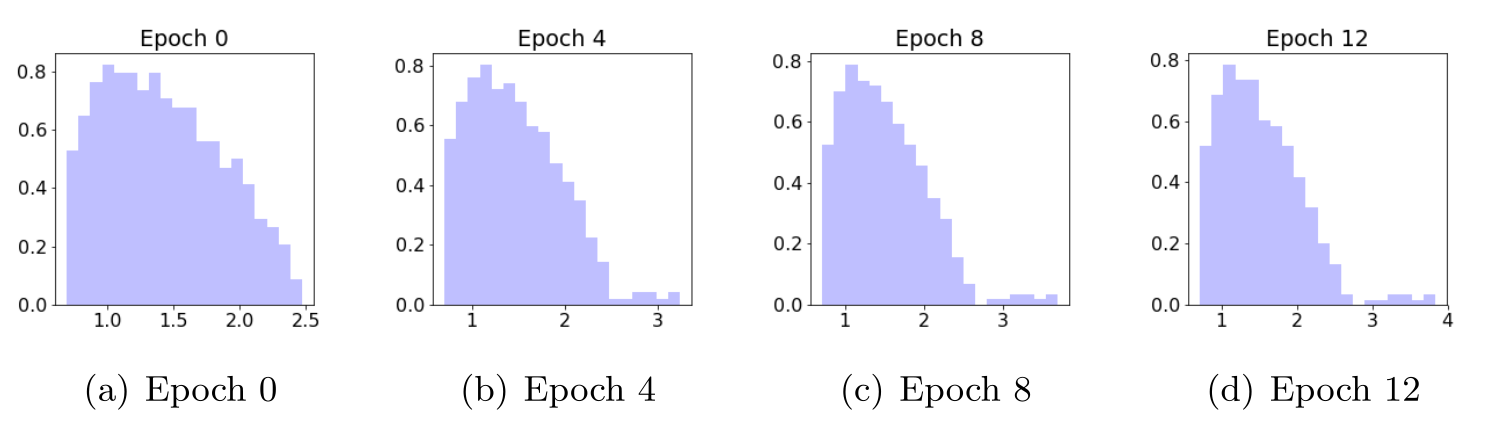
MiniAlexNet is trained on CIFAR-10 using two convolutional stages and fully connected layers, with SGD at learning rate 0.01 and momentum 0.9. The analyzed matrices include 4,096×384 and 384×192 layers. The baseline uses batch size 32 and up to 100 epochs, retaining weights at successive epochs. The first layer’s initially MP-like spectrum develops separated mass as training progresses, illustrated by all four panels in Figure 3.
Entropy and stable-rank measures decline while training accuracy rises, and the largest eigenvalue increases from roughly three to four in the illustrated sequence. Explicit L2 regularization or dropout strengthens some spectral separation and localization effects in the reported comparisons. These observations support the authors’ analogy between implicit and explicit regularization in this model; they do not establish that every declining rank statistic improves out-of-sample performance.
6 Explaining the Generalization Gap by Exhibiting the Phases
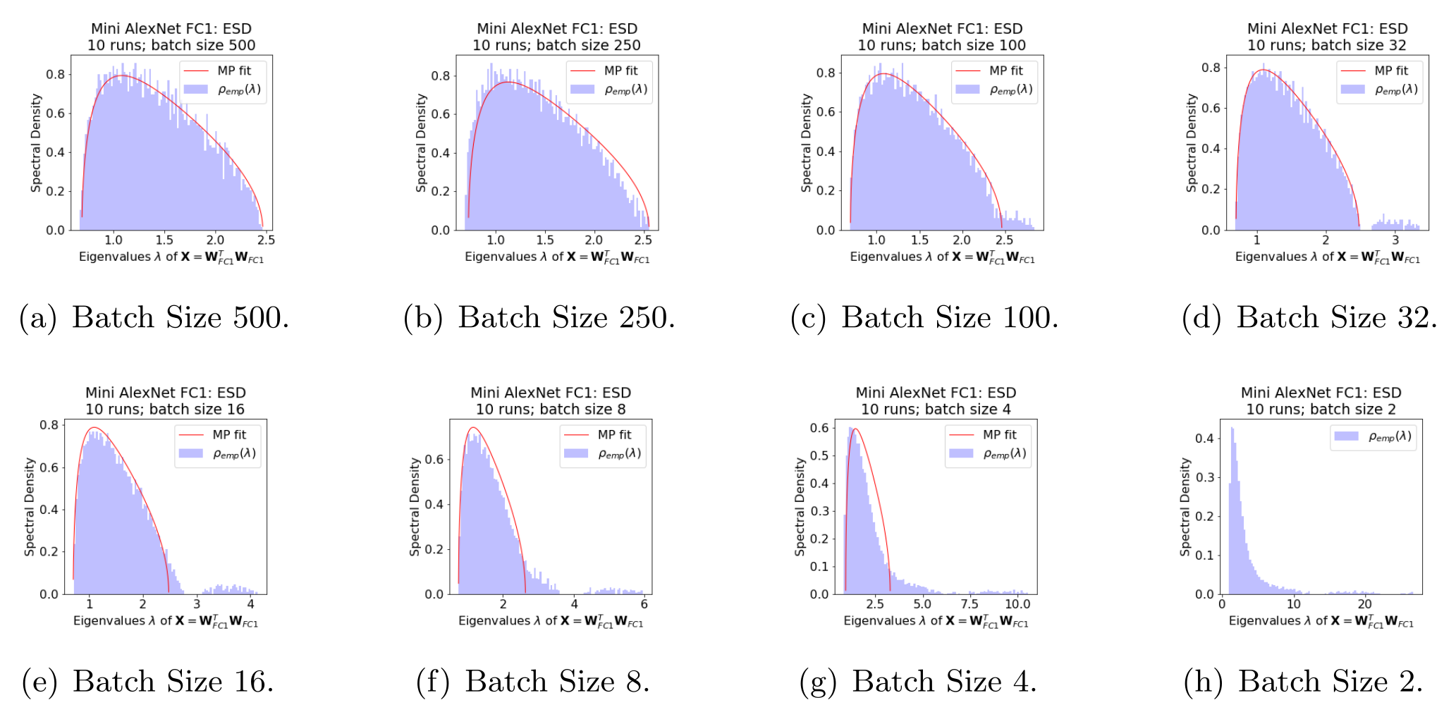
The batch-size sweep uses sizes 500, 250, 100, 50, 32, 16, 8, 4, and 2, with ten runs per setting. Figure 4 retains accuracy and rank summaries; Figure 5 shows eight representative spectra, omitting size 50. Large batches are mainly random-like, size 100 shows bleeding-out, size 32 develops bulk plus spikes, and smaller batches progress toward bulk decay and a heavy-tailed appearance. Test accuracy generally improves toward the smaller batches in this experiment, while training accuracy is comparatively flat at small sizes and deteriorates for sufficiently large batches.
The authors interpret the large-batch generalization gap as weaker implicit regularization and reduced learned correlations. The evidence is an association within this architecture, dataset, and training recipe. At fixed epochs, smaller batches also perform more optimizer updates, so this is not a matched-update or matched-compute comparison. It does not establish that all large-batch training must fail or that the spectral change is the sole causal mechanism. Nor do the displayed batch spectra independently demonstrate the additional rank-collapse regime.
7 Discussion and Conclusion
The proposed contribution is a practical spectrum-based framework for studying trained weight matrices without requiring training examples at inspection time. Its strongest evidence is the reported model spectra and controlled small-model sweeps. Extending the analysis to convolutional structures, larger architectures, predictive diagnostics, and a firmer theory of learned correlations remains open. Heavy-tailed fits and rank statistics should be treated as informative diagnostics with assumptions and finite-size limits, rather than certificates of generalization.