At a glance
CompILE learns reusable, variable-length behavior segments from state–action demonstrations. A differentiable segmentation model infers boundaries and latent codes, while subpolicies reconstruct the demonstrated actions. Grid-world and simulated reacher experiments test segmentation and longer task sequences; discovered grid-world skills also help hierarchical reinforcement learning under sparse rewards.
1 Introduction
The model jointly discovers where one behavior ends and what that behavior represents. After explaining one segment, it masks that portion of the trajectory and processes the remainder with shared parameters. This repeated structure supports new combinations and longer sequences. Segment labels are not required, although experiments provide the number of segments as weak supervision.
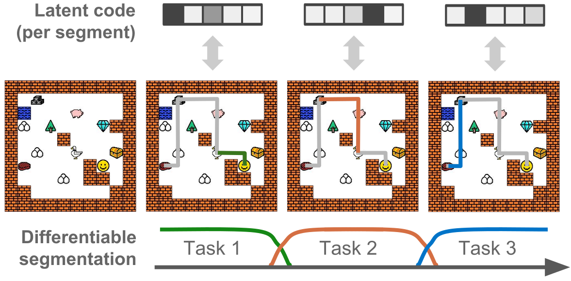
2 Model overview
A conditional variational autoencoder (VAE) represents each demonstrated state–action trajectory as a sequence of latent behavior codes and boundaries. The state sequence conditions reconstruction; the model learns which action to take at each state.
2.1 Behavioral cloning
Behavioral cloning (BC) maximizes the likelihood of expert actions given observed states. CompILE retains this imitation objective while dividing responsibility among latent subtask policies.
Equation 1
| (1) |
2.2 Sub-task identification and imitation
Boundaries partition a trajectory into at most M ordered segments, each controlled by a policy conditioned on its latent code. The model permits empty segments and categorical or continuous codes. A truncated Poisson-inspired boundary prior discourages both single-step fragmentation and one segment covering everything. The demonstrated environments are fully observable, and the decoder policy has no recurrent memory.
Equations 2–4
| (2) |
| (3) | ||||
| (4) |
2.2.1 Recognition model
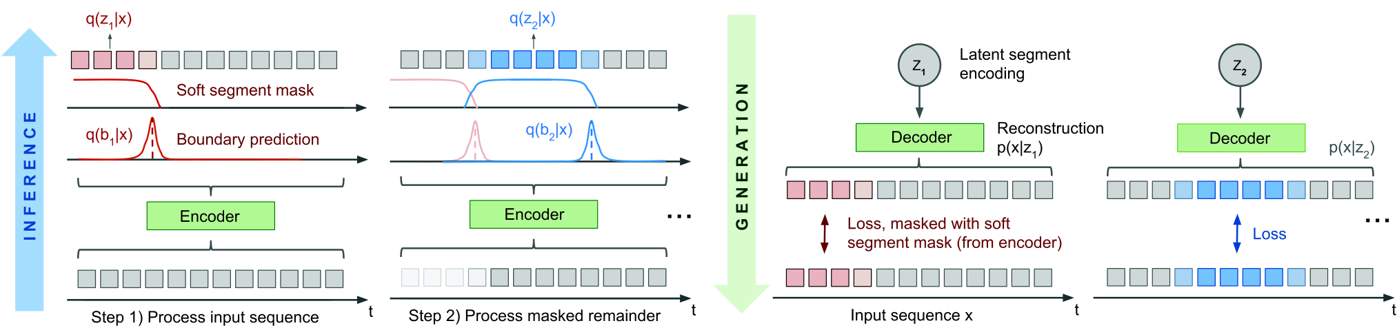
A shared long short-term memory (LSTM) encoder makes repeated passes over the trajectory. Separate output heads predict boundary positions and segment codes. Previously explained time steps are masked out, allowing the same inference process to operate on longer unseen sequences.
Equations 5–7
| (5) |
| (6) | ||||
| (7) |
2.2.2 Continuous relaxation
During training, Gumbel-softmax relaxations replace discrete boundary and code samples, enabling reparameterized gradients. Testing returns to discrete boundaries and codes.
Soft segment masks
Soft segment membership is computed from cumulative boundary probabilities. The lower boundary is the maximum of all earlier boundaries, so inconsistent relaxed predictions can yield empty segments. The resulting masks partition responsibility over time.
Equation 8
| (8) | ||||
RNN state masking
Each pass multiplies recurrent hidden and cell states by the probability that the current time step remains unexplained. This suppresses earlier segments while preserving gradients through boundary decisions.
Equation 9
| (9) | ||||
Soft RNN readout
Invalid boundary locations and padding are masked. Code logits are read as a boundary-weighted average of recurrent outputs, shifted by one time step because a boundary identifies the next segment’s start.
Equation 10
| (10) |
Loss masking
The action-reconstruction loss is weighted by each segment’s soft membership mask, so every subpolicy explains only its assigned portion of the demonstration. Training estimates the expected loss with one reparameterized posterior sample.
Equation 11
| (11) |
Number of segments
M is supplied during training and fixed across a minibatch. Giving the true number of subtasks is a form of weak supervision; the method does not automatically select an unrestricted number of segments.
Complexity
A forward pass costs O(TM) for trajectory length T and M segments, because inference and decoding revisit the sequence for every segment.
3 Related work
CompILE relates to option discovery, hierarchical imitation, sequence segmentation, and latent-variable models. It learns from offline demonstrations rather than requiring environment interaction during skill discovery. Unlike task-sketch approaches such as TACO, the main model need not receive subtask identities or their order. Its latent codes can be discrete or continuous.
4 Experiments
Experiments ask whether the model discovers useful boundaries and codes, generalizes from three to five subtasks, and provides useful actions for a hierarchical reinforcement learning agent.
4.1 Multi-task environments
Both environments are fully observable simulations with generated demonstrations and known evaluation boundaries.
Grid world
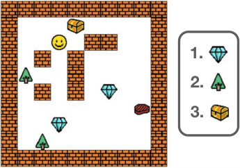
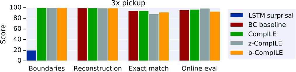
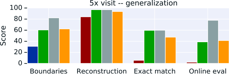
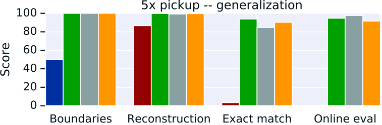
A 10×10 grid contains walls and objects. Tasks visit or pick up specified object types in sequence; demonstrations follow shortest paths. Training uses three-task sequences, while testing includes five-task sequences and new layouts.
Continuous control
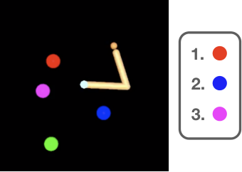
A two-link reacher touches a sequence of colored targets. Observations give target locations and arm state, and a hand-written controller generates demonstrations. Tasks contain three or five target reaches.
4.2 Imitation learning
The model trains on three-task demonstrations with Adam, batch size 256, and learning rate 0.0001. Grid-world training uses 50,000 iterations and reacher training 500,000. A separate causal termination policy learns the inferred boundaries without future observations. Evaluation uses 1,024 new instances and supplies M=3 or M=5 according to the test sequence.
Baselines
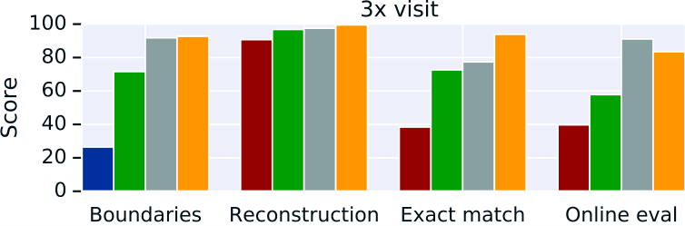
Baselines include an LSTM that detects surprising actions and a single-segment VAE behavioral-cloning model. Partially supervised variants provide code identities (z-CompILE) or boundaries (b-CompILE) during training; these labels are not supplied at test time.
Grid world results
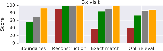
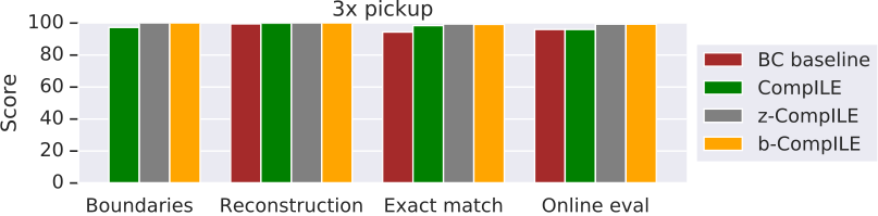
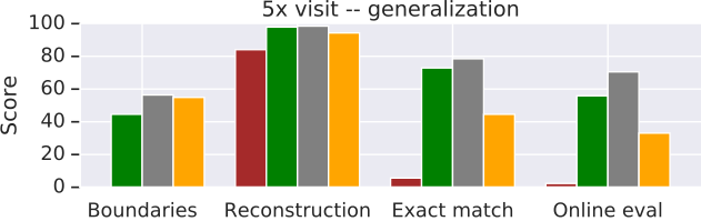
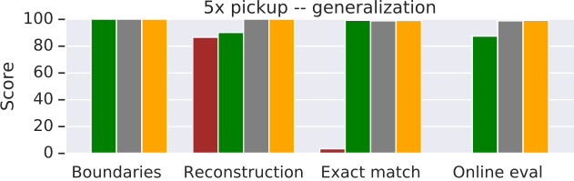
Pickup boundaries and reconstructions are accurate, including on longer sequences; the single-segment baseline generalizes poorly. Visit tasks are more ambiguous because an agent can accidentally pass over an object, which can confuse termination. Reconstruction given expert states and successful online execution are reported separately.
Continuous control results
Unsupervised CompILE improves reacher boundary detection over the surprisal baseline but often misses the exact generating segmentation. Allowing a one-step boundary tolerance improves some scores, while partial supervision yields much stronger results. The paper does not report continuous-control reconstruction or execution performance because behavioral-cloning covariate shift remains unresolved.
| Model | Accuracy | F1 (tol=0) | F1 (tol=1) |
|---|---|---|---|
| 3 tasks | |||
| LSTM surprisal | |||
| CompILE | |||
| z-CompILE | |||
| b-CompILE | |||
| 5 tasks – generalization | |||
| LSTM surprisal | |||
| CompILE | |||
| z-CompILE | |||
| b-CompILE | |||
4.3 Hierarchical reinforcement learning
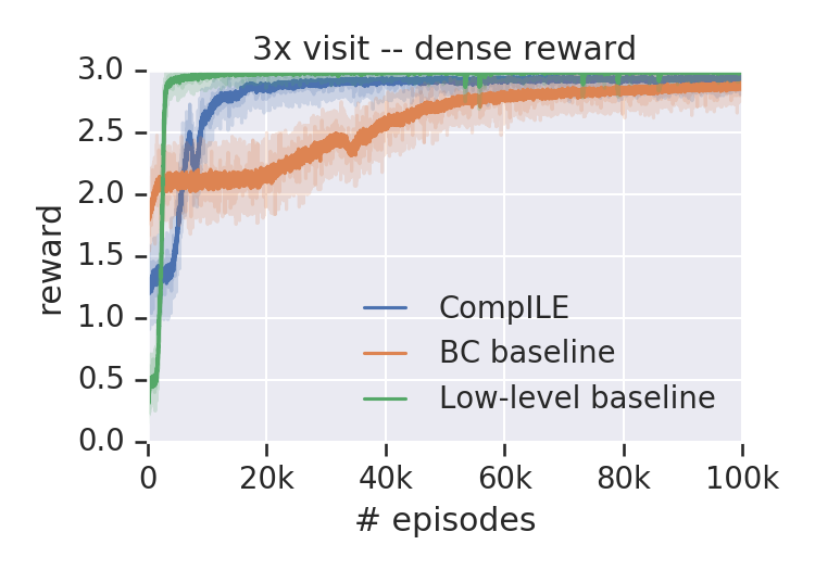
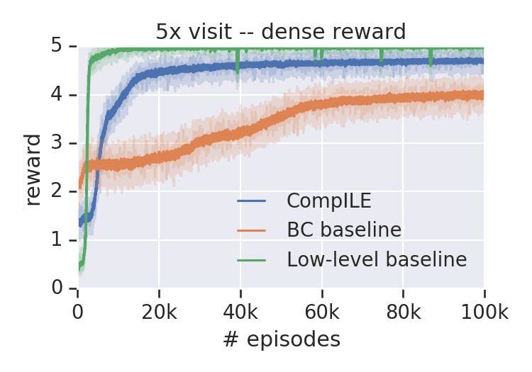
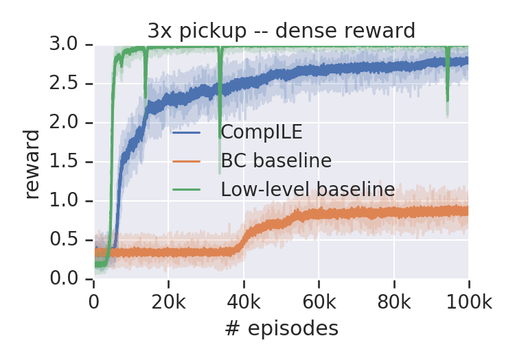
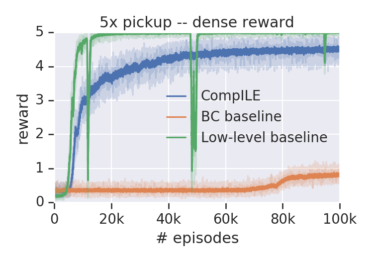
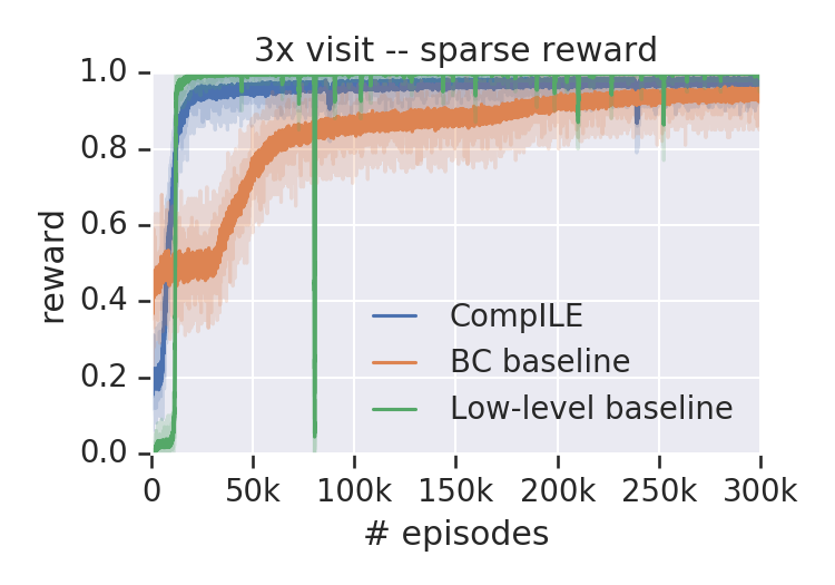
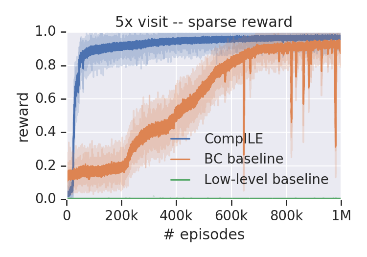
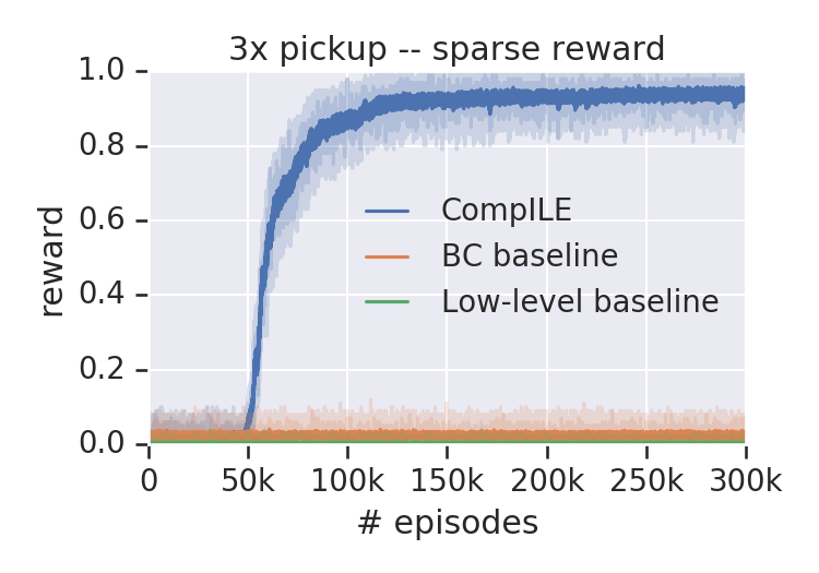
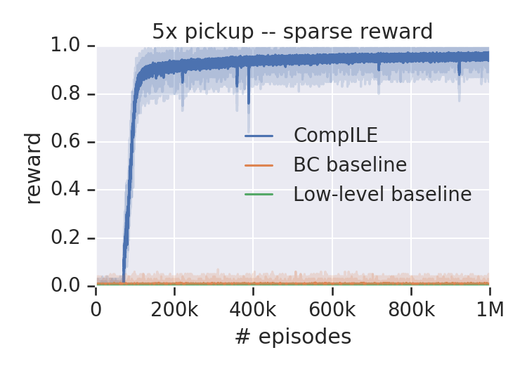
A hierarchical IMPALA agent chooses either primitive actions or pretrained CompILE skills with learned termination. It solves sparse-reward pickup tasks that the tested flat and single-segment baselines struggle with, including five-task compositions after three-task pretraining. With dense subtask rewards, the flat baseline can learn with fewer episodes. These results concern grid-world control, not the reacher or a physical robot.
4.4 Limitations and future work
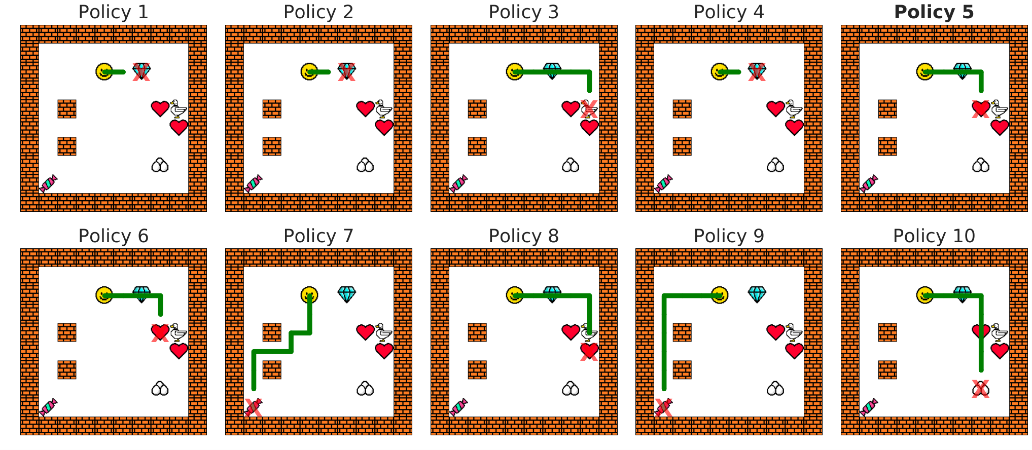
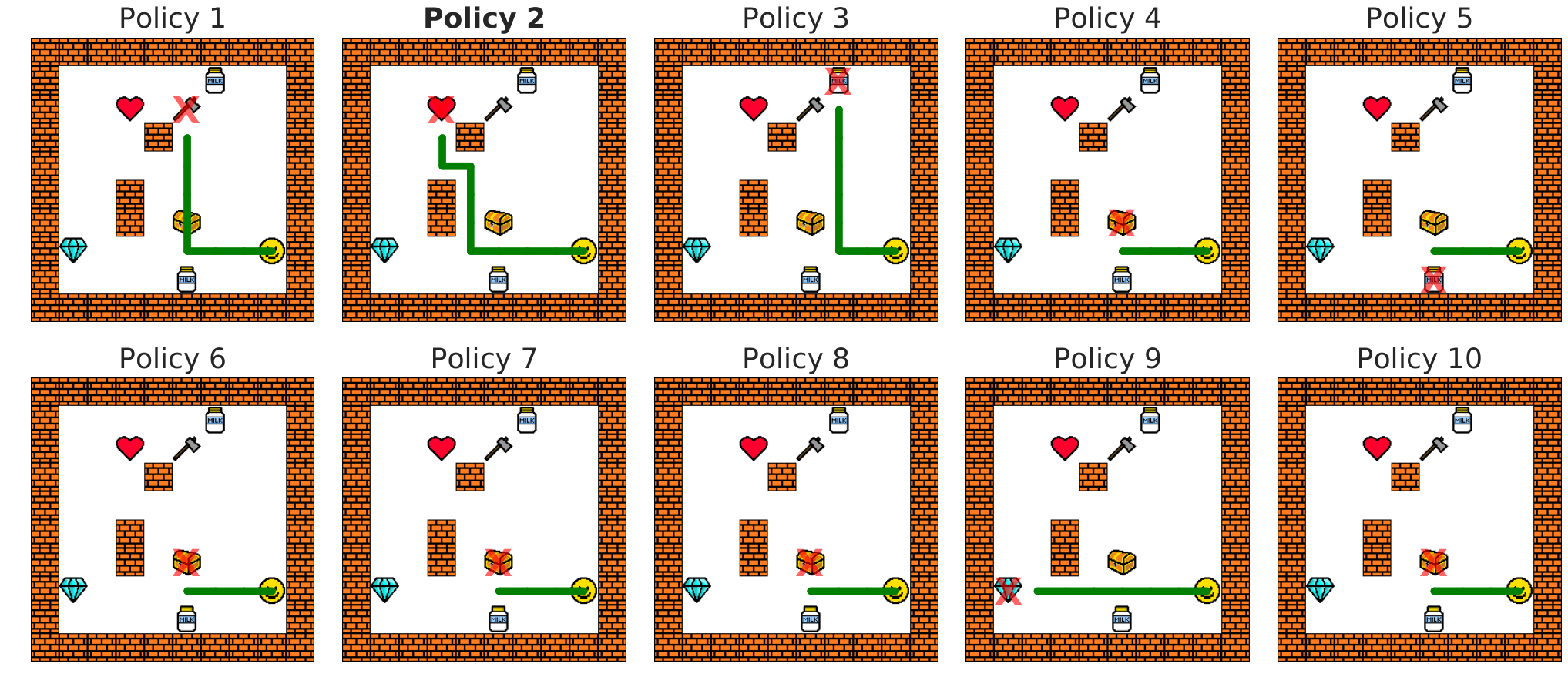
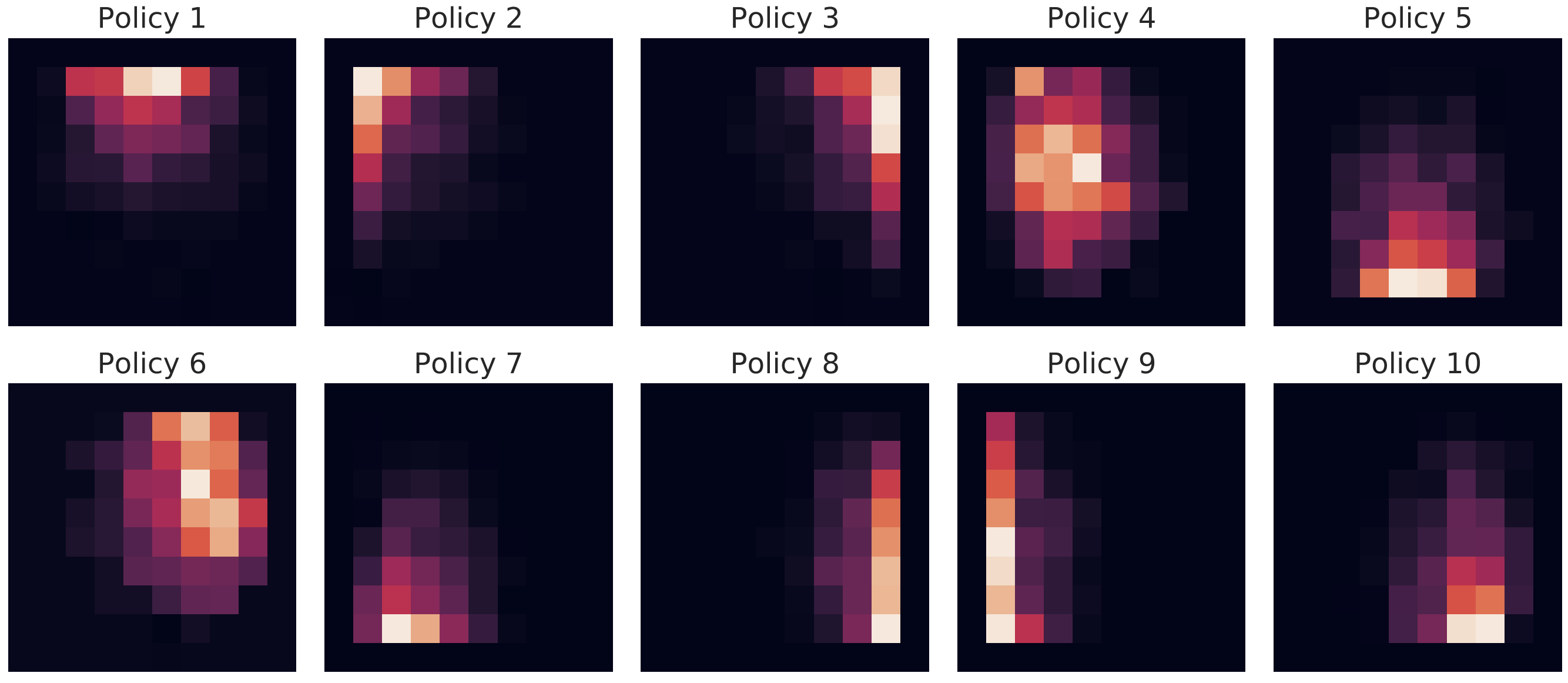
Discovered codes need not correspond to human task labels: the model often learns location-based rather than object-based skills. The number of segments supplies weak supervision, and partially observable environments would require decoder memory and mechanisms preventing it from ignoring latent codes.
5 Conclusions
Joint segmentation and imitation can yield reusable skills for longer compositions and sparse-reward learning. Applications to other sequential data, episodic memory, partial observability, and higher-level planning remain proposed extensions.
Acknowledgements
The authors acknowledge colleagues for discussions and feedback.
Appendix A CompILE model details
The appendix specifies architectures, termination, variational training, alternative latent codes, and sensitivity to segmentation settings.
A.1 Encoder architecture
The encoder converts observations and actions into recurrent inputs; its state is reset between trajectories and segment passes.
Grid world
Grid observations pass through two 3×3 convolutional layers with 64 feature maps, followed by a linear projection and layer normalization. The recognition network additionally receives an action embedding.
Continuous control environment
For continuous control, a two-layer perceptron with 256 hidden units per layer replaces the convolutional encoder.
A.2 Sub-task policies
Discrete codes select separate policy heads sharing the visual encoder. A soft mixture supplies gradients during relaxed training. This design generalizes better in initial experiments than feeding an embedded categorical code into one shared policy.
A.3 Termination policy
A separate recurrent termination network learns to mark the boundary predicted by the inference model. During execution it terminates a skill when its sigmoid output exceeds 0.5.
A.4 ELBO objective for learning
The evidence lower bound (ELBO) combines action reconstruction with a Kullback–Leibler (KL) penalty between posterior and prior. The retained derivation follows from Jensen’s inequality, and Figure 6 shows the graphical model.
Equations 12–13
| (12) |
| (13) |
A.5 KL term
A coefficient β controls prior regularization. Training uses categorical KL terms even for relaxed samples. Because exact previous boundaries are unavailable, the boundary-prior term is evaluated for the first boundary and multiplied by M, relying on shared segment-distribution assumptions.
A.6 Gaussian latent variables
A variant replaces categorical codes with 32-dimensional Gaussian variables and uses one code-conditioned decoder. The appendix reports grid-world and reacher segmentation results for this alternative.
| Model | Accuracy | F1 (tol=0) | F1 (tol=1) |
|---|---|---|---|
| 3 tasks | |||
| LSTM surprisal | |||
| CompILE | |||
| z-CompILE | |||
| b-CompILE | |||
| 5 tasks – generalization | |||
| LSTM surprisal | |||
| CompILE | |||
| z-CompILE | |||
| b-CompILE | |||
A.7 Attentive readout
An alternative attention head reads code information from any point within the softly masked segment. Results are similar to final-step readout in these tasks, with attention often focusing near the segment end.
Equations 14–15
| (14) |
| (15) |
A.8 Other hyperparameters
The following settings and ablations explain the model’s sensitivity to capacity, segment count, and relaxation temperature.
Number of hidden units and MLP layers
Most perceptron and LSTM layers have 256 hidden units. Boundary prediction uses a hidden-layer perceptron, code prediction a linear head, and the termination head two hidden layers. Smaller networks mainly reduce reconstruction quality.
Number of segments
Providing the true number of segments generally works best. Extra segments sometimes collapse to the sequence end but can also split one behavior unnecessarily, slightly reducing boundary accuracy.
Poisson prior rate
All experiments use Poisson rate λ=3; the authors report limited sensitivity to its precise value.
Softmax temperature
Reported experiments usually fix Gumbel-softmax temperature at 1. Annealing can help, whereas starting with a lower fixed temperature reduces unsupervised boundary accuracy in the tested reacher settings.
Appendix B Reinforcement learning agent details
The hierarchical reinforcement learning experiments reuse pretrained skills and train a task-conditioned controller over them.
B.1 Architecture and hyperparameters
The controller uses a smaller convolutional network and 128-unit perceptron layers. It can call ten learned skills or primitive actions; the single-segment comparison uses a larger categorical code space. Task embeddings condition both the image encoder and policy head. Adam uses learning rate 0.001 and batch size 256; discounting is 0.99.
B.2 Distributed training
IMPALA distributes environment interaction among CPU actors and learning to a GPU learner. Off-policy correction accounts for actor trajectories generated with older policy parameters.
Appendix C Environment implementation details
The environment specifications describe observations, demonstrations, task construction, and episode limits.
C.1 Grid world
The grid world provides four movement and four directional pickup actions, with a 10×10×12 observation tensor. Random mazes are simplified by wall subsampling and checked for solvable tasks. Breadth-first search generates demonstrations, truncated at 42 steps during training and 200 during testing.
C.2 Continuous control
The simulated reacher has two links of length 0.12 and targets of diameter 0.05. A 32-dimensional observation records ten targets’ visibility and coordinates plus two joint angles. Episodes last at most 100 control steps. The demonstration controller independently adjusts shoulder direction and elbow opening toward the current target.
Appendix D Evaluation details
Evaluation distinguishes segmentation, reconstruction under expert observations, and execution in the environment.
D.1 Metrics
Boundary accuracy checks exact task transitions; F1 also evaluates unordered boundary matches with optional one-step tolerance. Reconstruction measures per-action agreement and exact full-sequence agreement while using expert states. Online evaluation executes inferred skills with learned termination and reports complete-task success, allowing errors to affect subsequent observations.
Equations
D.2 Segmentation baseline (LSTM surprisal)
The LSTM-surprisal baseline marks the M−1 least-likely demonstrated actions as boundaries. It shares comparable encoders and is trained only on three-task sequences. Its stronger pickup boundary detection on five-task sequences may reflect surprise at events absent during training rather than learned reusable structure.
Equations 16–17
| (16) |
| (17) |
Appendix E Qualitative results
The retained qualitative figures visualize each discovered policy, its chosen object, and its termination location. They show that codes often partition space rather than encode object identity, although the model can distinguish nearby objects in some scenes.