At a glance
GPipe partitions a sequential model across accelerators, divides each minibatch into microbatches, and pipelines their execution. Gradients accumulate before one synchronous update, while activation recomputation saves memory. Demonstrations include a 557-million-parameter image classifier and a six-billion-parameter multilingual Transformer. This edition uses the circulated arXiv manuscript plus the official conference supplement; the proceedings title is “GPipe: Efficient Training of Giant Neural Networks using Pipeline Parallelism.”
1 Introduction
Larger models can improve quality but exceed individual-device memory. GPipe provides a layer-sequence interface instead of a task-specific parallelization scheme. Pipeline stages handle different microbatches concurrently; a synchronized minibatch update avoids stale weights. Data parallelism can be added around the pipeline.
2 The GPipe Library
The implementation is a Lingvo library, but the partitioning and execution ideas are independent of that framework.
2.1 Interface
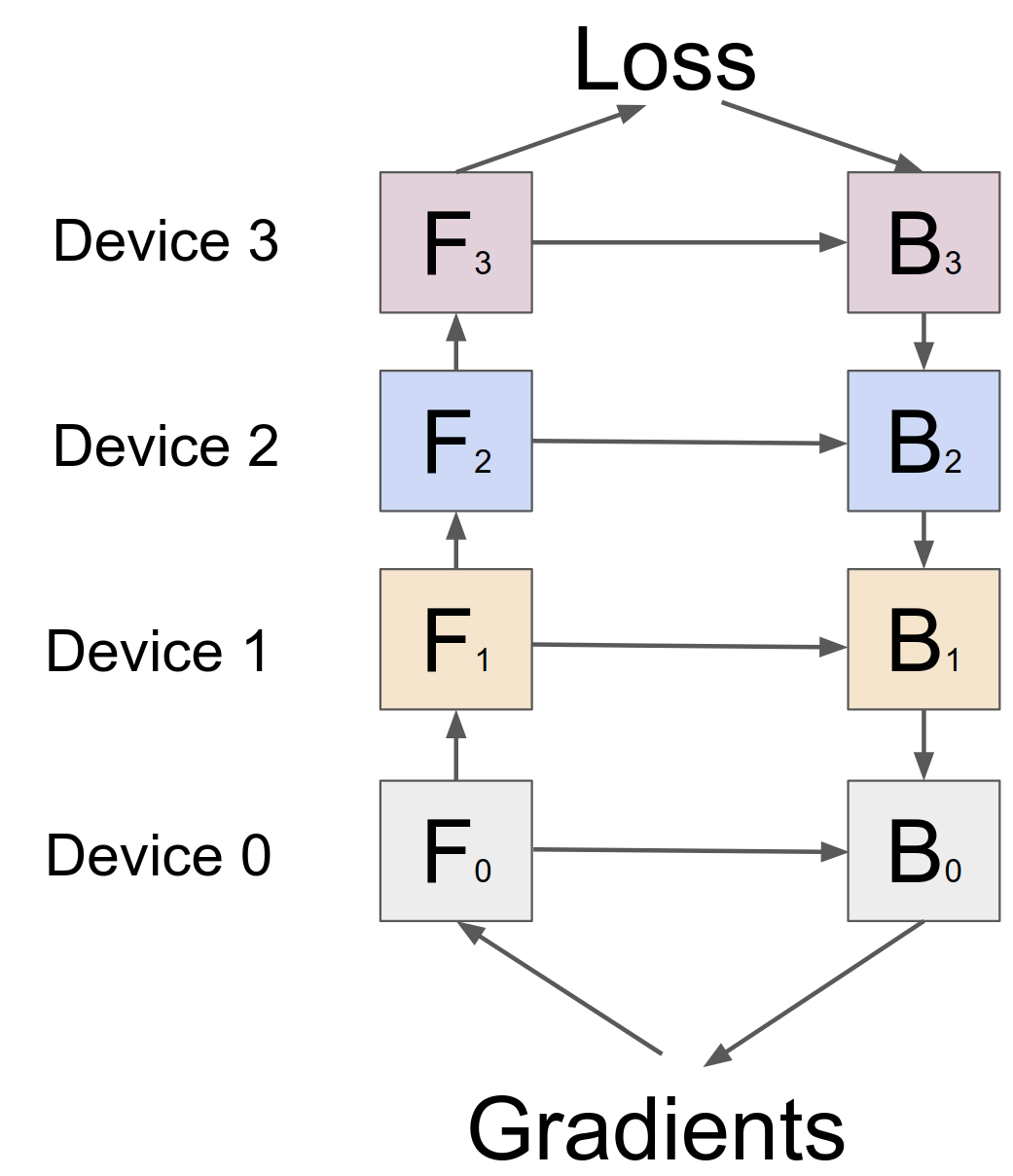
Users supply a sequence of layers, the number of partitions, and the number of microbatches. Optional layer-cost estimates guide grouping adjacent layers into balanced stages. Each stage has a composite forward function and automatically differentiated backward computation.
2.2 Algorithm
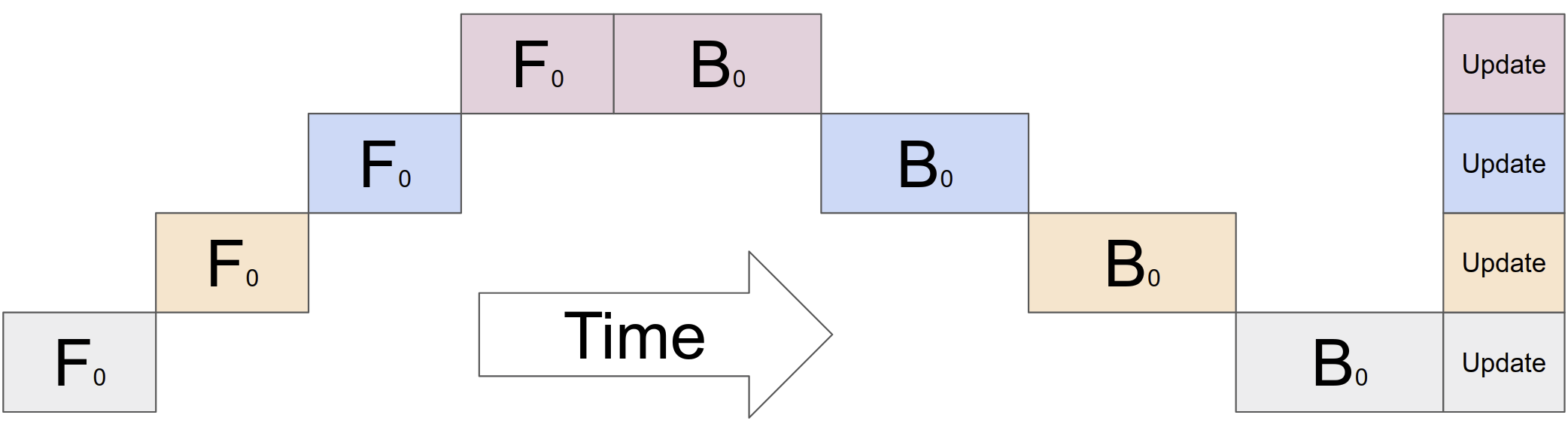
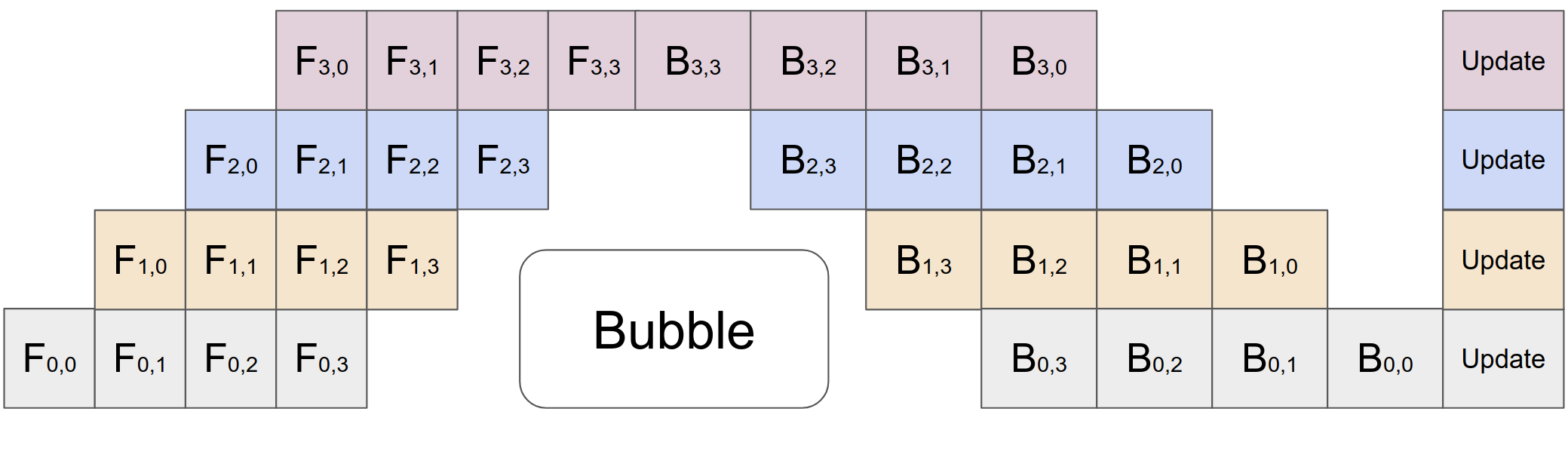
A minibatch is split into equal microbatches. Each travels through consecutive stages, with communication only at stage boundaries. Backpropagation uses the same weights as its forward pass; all microbatch gradients accumulate before an update. Batch normalization is a special case: training statistics use microbatches, while evaluation statistics aggregate across the minibatch.
2.3 Performance Optimization
Recomputation stores boundary activations and rebuilds intermediate values during backpropagation. This saves memory at extra compute cost. Pipeline fill/drain bubbles shrink as microbatch count grows; the experiments find overhead small when there are at least four times as many microbatches as stages. Uneven layer cost or memory can still leave stages underutilized.
3 Performance Analyses
Recomputation alone fits substantially larger models on one accelerator. Partitioning supports a 1.8-billion-parameter AmoebaNet and an 83.9-billion-parameter Transformer in capacity tests; these are distinct from the trained quality demonstrations. Throughput approaches linear scaling for balanced Transformer layers, while uneven AmoebaNet stages scale less well. Tests without fast interconnects still improve because communication is limited to boundary activations.
| NVIDIA GPUs (8GB each) | Naive-1 | Pipeline-1 | Pipeline-2 | Pipeline-4 | Pipeline-8 |
|---|---|---|---|---|---|
| AmoebaNet-D (L, D) | (18, 208) | (18, 416) | (18, 544) | (36, 544) | (72, 512) |
| # of Model Parameters | 82M | 318M | 542M | 1.05B | 1.8B |
| Total Model Parameter Memory | 1.05GB | 3.8GB | 6.45GB | 12.53GB | 24.62GB |
| Peak Activation Memory | 6.26GB | 3.46GB | 8.11GB | 15.21GB | 26.24GB |
| Cloud TPUv3 (16GB each) | Naive-1 | Pipeline-1 | Pipeline-8 | Pipeline-32 | Pipeline-128 |
| Transformer-L | 3 | 13 | 103 | 415 | 1663 |
| # of Model Parameters | 282.2M | 785.8M | 5.3B | 21.0B | 83.9B |
| Total Model Parameter Memory | 11.7G | 8.8G | 59.5G | 235.1G | 937.9G |
| Peak Activation Memory | 3.15G | 6.4G | 50.9G | 199.9G | 796.1G |
| TPU | AmoebaNet | Transformer | ||||
|---|---|---|---|---|---|---|
| 2 | 4 | 8 | 2 | 4 | 8 | |
| 1 | 1.13 | 1.38 | 1 | 1.07 | 1.3 | |
| 1.07 | 1.26 | 1.72 | 1.7 | 3.2 | 4.8 | |
| 1.21 | 1.84 | 3.48 | 1.8 | 3.4 | 6.3 | |
4 Image Classification
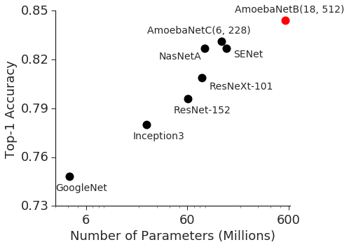
A four-stage, 557-million-parameter AmoebaNet trained at 480-pixel resolution reaches 84.4% ImageNet top-one and 97.0% top-five single-crop validation accuracy. Fine-tuning improves several transfer datasets, including 99.0% CIFAR-10 and 91.3% CIFAR-100 accuracy. The comparison table marks systems using additional private pretraining data.
| Dataset | # Train | # Test | # Classes | Accuracy () | Previous Best () |
|---|---|---|---|---|---|
| ImageNet-2012 | 1,281,167 | 50,000 | 1000 | [12] ([27]) | |
| CIFAR-10 | 50,000 | 10,000 | 10 | [26] | |
| CIFAR-100 | 50,000 | 10,000 | 100 | [26] | |
| Stanford Cars | 8,144 | 8,041 | 196 | [26] | |
| Oxford Pets | 3,680 | 3,369 | 37 | [29] | |
| Food-101 | 75,750 | 25,250 | 101 | [30] | |
| FGVC Aircraft | 6,667 | 3,333 | 100 | [31] | |
| Birdsnap | 47,386 | 2,443 | 500 | [32] |
5 Massive Massively Multilingual Machine Translation
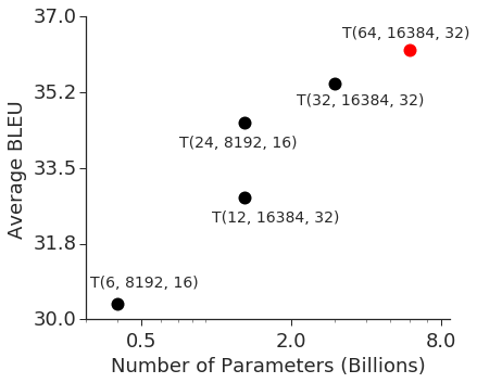
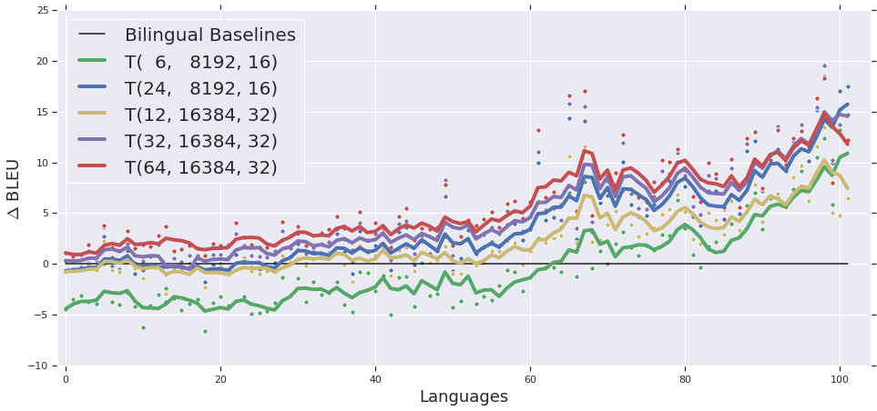
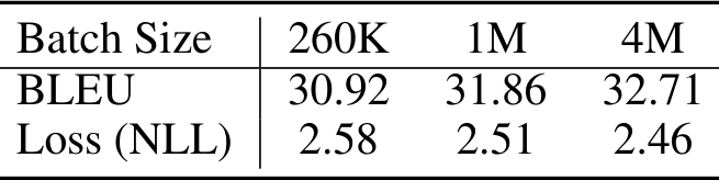
A shared multilingual model is trained on 102 languages paired with English. Increasing capacity from roughly 400 million to six billion parameters improves translation, with diminishing returns. At equal parameter count, deeper models particularly help low-resource languages. Deep training needs scaled initialization and clipped logits to avoid unstable gradients. Increasing effective batch size to four million tokens improves the reported German–English metrics; this is an empirical result for this setup.
6 Design Features and Trade-Offs
Tensor partitioning can scale individual layers but adds frequent collective communication. Asynchronous pipelines improve utilization but face weight-staleness and version-storage costs. GPipe trades a fill/drain bubble and activation recomputation for synchronous updates and low communication. Every individual layer must still fit on one accelerator, and batch-dependent operations need special handling.
7 Conclusion
The main result is a practical way to scale model memory and training across devices with predictable synchronous optimization. Efficiency depends on balanced stages and enough microbatches; larger capacity and measured throughput do not guarantee improved task quality by themselves.
Supplement 1: example usage
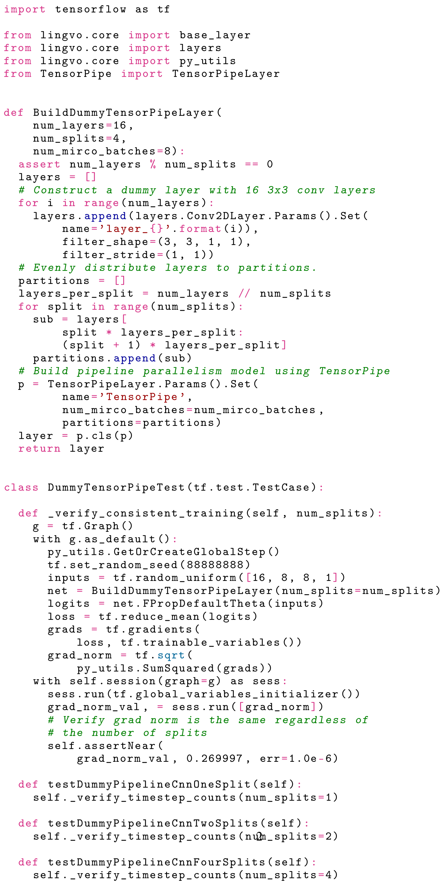
The official supplement illustrates composing layer sequences and checking gradient-norm consistency across partition counts. The complete original code panel is retained as printed, including its historical TensorPipe names and typographical inconsistencies.
Supplement 2.1: image-training settings
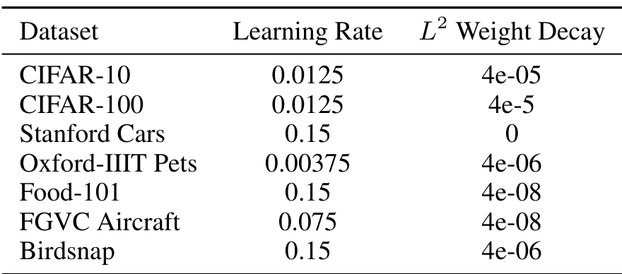
AmoebaNet training uses RMSProp, label smoothing, an auxiliary classification head, drop-path regularization, and final-layer dropout. Transfer-learning rates and weight decay are chosen using a 20% training holdout and rerun five times with the selected settings. The original table gives each dataset’s chosen values.
Supplement 2.2: training consistency
AmoebaNet-D is trained repeatedly for 35 epochs. Runs with one, two, four, and eight partitions finish within 1.6 standard deviations of the mean accuracy of five baseline runs, supporting consistency within observed training variation.
Supplement 3: translation data
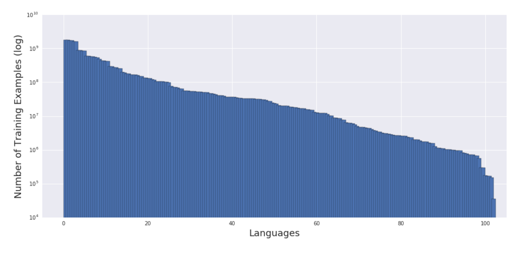
The original plot shows the strong imbalance across 102 language pairs, from roughly 35,000 to two billion training examples. The dataset is assembled from parallel web sentences.
Supplement 3.1: bilingual baselines
Bilingual Transformer models use a shared 32,000-token source/target vocabulary, tuned dropout, and Adafactor with warm-up and inverse-square-root learning-rate decay. Checkpoints are selected by validation performance; translation scores use the reported true-cased evaluation setup.
Supplement 3.2: multilingual sampling
Temperature-based sampling balances high-resource performance against transfer to low-resource languages. Sampling probabilities are proportional to the fifth root of each language pair’s natural corpus probability. The multilingual model shares a 64,000-token vocabulary generated under the same distribution.
Supplement 3.3: large batches
The retained table repeats the German–English comparison: increasing the token batch from 260,000 to four million improves both translation score and likelihood in this training setup. It does not establish a universal benefit from larger batches.
Supplement 4: depth and generalization
At comparable parameter counts, deeper translation models particularly improve low-resource languages. The original convergence plot also shows faster optimization with increased depth under controlled batch size, width, and optimizer settings. These empirical observations motivate further study; diminishing returns and training instability remain limitations.