Literature
Display
← All papers

Constrained Exploration and Recovery from Experience Shaping

Pham, Tu-Hoa · De Magistris, Giovanni · Agravante, Don Joven · Chaudhury, Subhajit · Munawar, Asim · Tachibana, Ryuki

· arXiv (preprint) ↗

Robotics4 min text · CondensedOriginal paper ↗
Contents

Overview

At a glance

CERES learns state-dependent constraints on a policy’s actions from positive and negative experience, then projects proposed actions into the predicted admissible region. A separate recovery policy helps label uncertain experience by testing whether the agent can remain alive. Simulated navigation experiments show better learning and rewards than the tested PPO baseline, including when the main policy receives fewer observations. The learned labels and constraints are approximate, so the method does not certify safety during exploration.

1 Introduction

Reward penalties can make exploration either reckless or excessively conservative. Instead of learning only a reward or an imitation policy, this paper uses demonstrations to learn which actions should be disallowed. Its supervised component separates positive from negative state–action pairs; CERES then generates these examples while learning the task and a recovery behavior. The authors’ implementation accompanies the work.
Refer to caption
Refer to caption
Refer to caption
Refer to caption
Refer to caption
Refer to caption
Refer to caption
Refer to caption
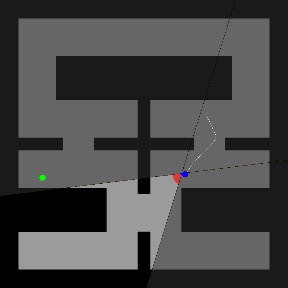
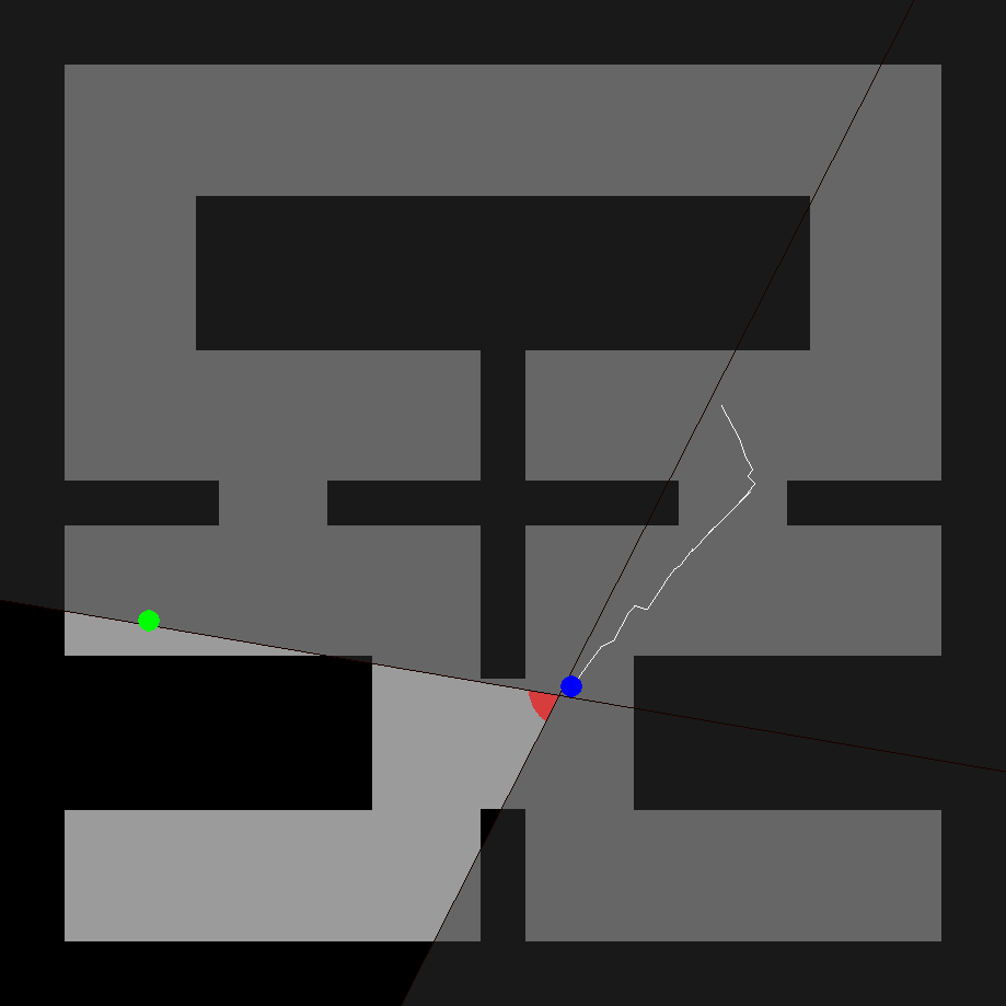
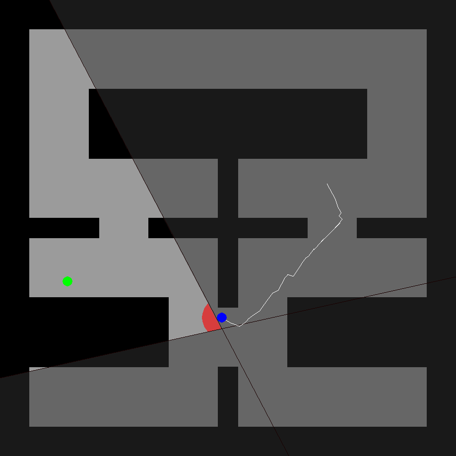
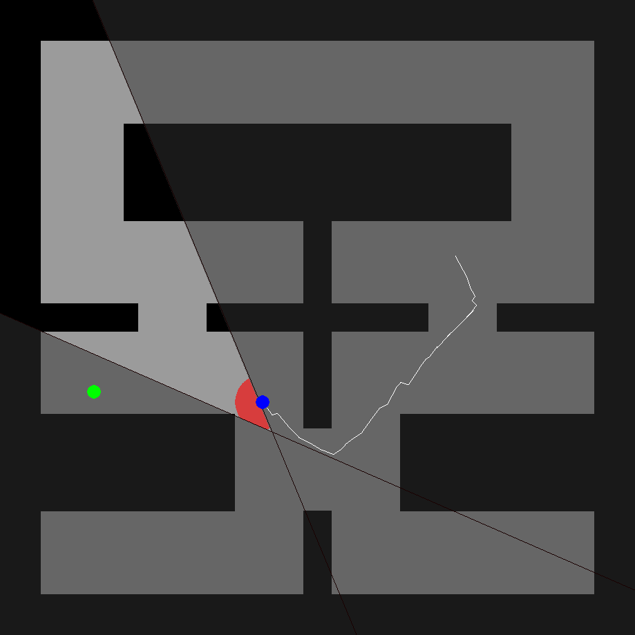
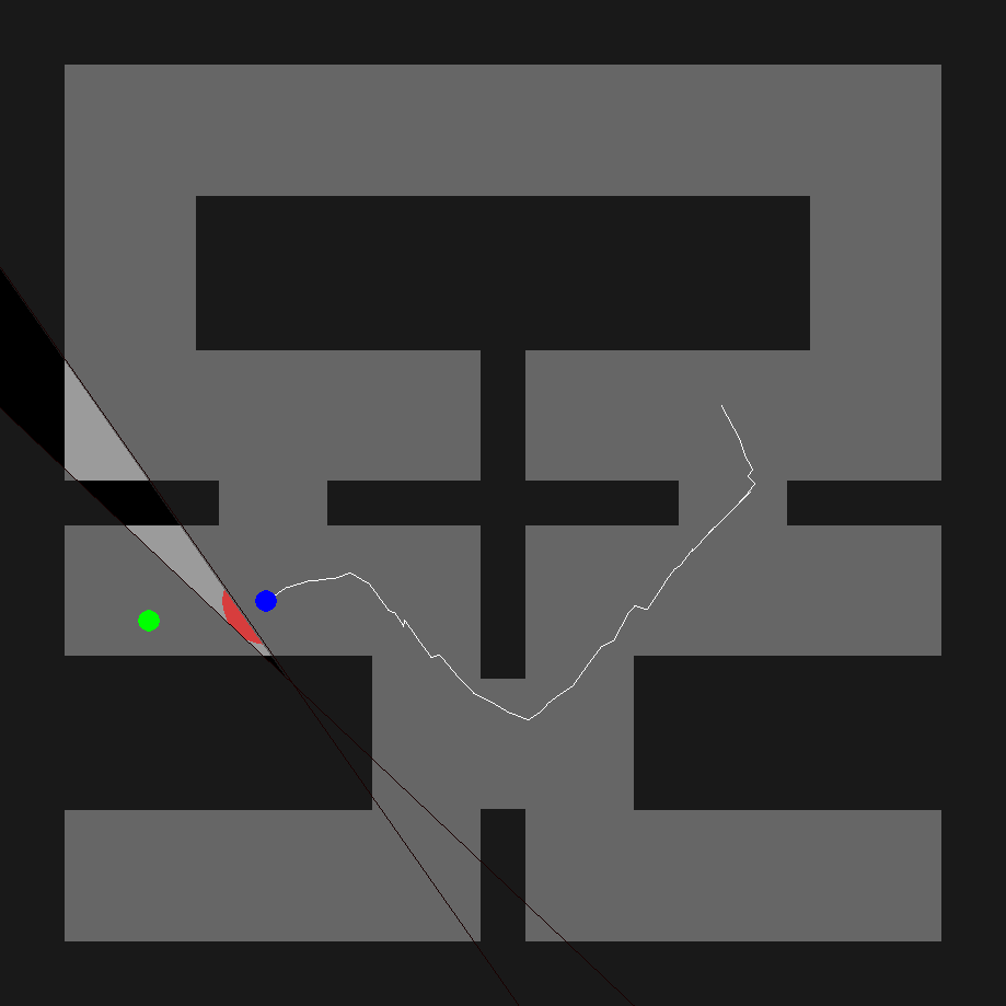
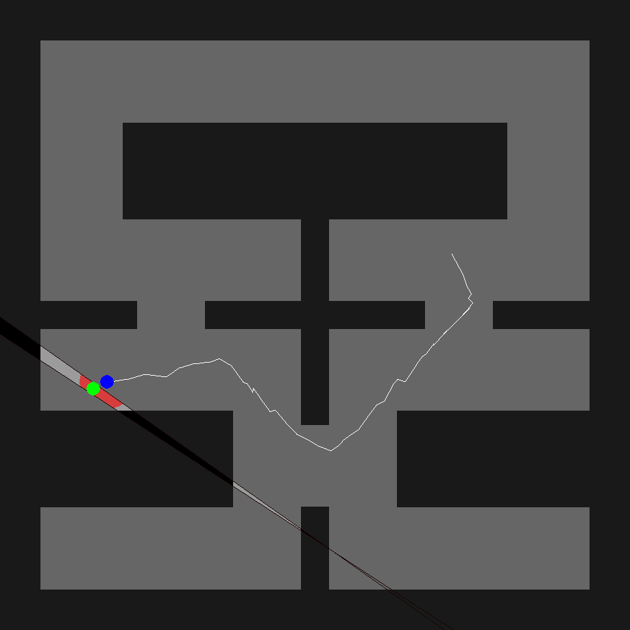
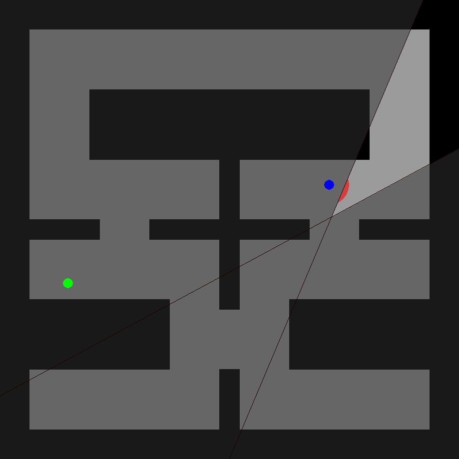
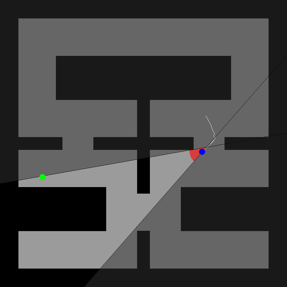
Figure 1: From left to right, top to bottom: consecutive actions taken during reinforcement learning in a maze environment with safety constraints. While in the unconstrained setting, the agent is permitted to take steps anywhere within the red circle, our approach learns safety constraints (shaded area) preventing failure from hitting obstacles (black surfaces).

2 Background and Motivation

2.1 Reinforcement Learning

The setting is a discounted Markov decision process with continuous actions. A neural Gaussian policy is optimized with PPO using environment trajectories. Safety constraints are learned separately from the reward-driven task policy, reducing reliance on a carefully balanced collision penalty. [26]

Equation 1
η⁡(π)=𝔼τ[∑i=0∞γi​R​(𝐬i,𝐱i,𝐬i+1)],\displaystyle\eta{\left({\pi}\right)}=\mathop{\mathbb{E}}\limits_{\tau}{\left[{\sum\limits_{i=0}^{\infty}{\gamma^{i}R{\left({\mathbf{s}_{i},\mathbf{x}_{i},\mathbf{s}_{i+1}}\right)}}}\right]}, (1)

2.2 Safe Reinforcement Learning

A quadratic program changes the proposed action as little as possible while satisfying linear inequalities. Earlier approaches supply these inequalities manually; here a network predicts them from the current state. Positive examples preserve the possibility of recovery, negative examples lead to failure, and uncertain examples require further investigation. Finite recovery trials are a heuristic for these labels, not proof that recovery is impossible. [22]

Equation 2
𝐱∗=argmin𝐱∈ℝnact{‖𝐱−𝐱~‖2such that𝐆𝐱≤𝐡},\displaystyle\mathbf{x}^{*}=\mathop{\text{argmin}}\limits_{\mathbf{x}\in\mathbb{R}^{{{n_{\text{act}}}}}}{\left\{{{\left\lVert{\mathbf{x}-\widetilde{\mathbf{x}}}\right\rVert}^{2}\enskip\text{such that}\enskip\mathbf{G}\mathbf{x}\leq\mathbf{h}}\right\}}, (2)

3 Learning Action-Space Constraints from Positive and Negative Demonstrations

3.1 Definitions

State-dependent action-space constraints

Each inequality defines a half-space in action coordinates. The constraint network predicts its normal and offset from the observed state. Satisfaction and violation margins measure which side of each boundary an action occupies; their geometric interpretation becomes useful after normalizing each normal vector.

Equations 3–8
ci​(𝐱)≤0,i∈[1,nin].\displaystyle c_{i}{{\left({\mathbf{x}}\right)}}\leq 0,\quad i\in\left[1,{n_{\text{in}}}\right]. (3)
ci​(𝐱)=𝐠i​𝐱−hi,i∈[1,nin].\displaystyle c_{i}{{\left({\mathbf{x}}\right)}}=\mathbf{g}_{i}\mathbf{x}-h_{i},\quad i\in\left[1,{n_{\text{in}}}\right]. (4)
𝐆𝐬​𝐱≤𝐡𝐬,with​(𝐆𝐬,𝐡𝐬)=𝒩C​(𝐬).\displaystyle\mathbf{G}^{\mathbf{s}}\mathbf{x}\leq\mathbf{h}^{\mathbf{s}},\enskip\text{with}\enskip{\left({\mathbf{G}^{\mathbf{s}},\mathbf{h}^{\mathbf{s}}}\right)}=\mathcal{N}^{C}{{\left({\mathbf{s}}\right)}}. (5)
ci𝐬​(𝐱)=𝐠i𝐬​𝐱−hi𝐬,i∈[1,nin],\displaystyle c_{i}^{\mathbf{s}}{{\left({\mathbf{x}}\right)}}=\mathbf{g}_{i}^{\mathbf{s}}\mathbf{x}-h_{i}^{\mathbf{s}},\quad i\in\left[1,{n_{\text{in}}}\right], (6)
MiS​(𝐬,𝐱)=max⁡(0,−ci𝐬​(𝐱))=ReLU⁡(−ci𝐬​(𝐱)),\displaystyle M^{S}_{i}{{\left({\mathbf{s},\mathbf{x}}\right)}}=\max{\left({0,-c_{i}^{\mathbf{s}}{{\left({\mathbf{x}}\right)}}}\right)}=\Arelu{\left({-c_{i}^{\mathbf{s}}{{\left({\mathbf{x}}\right)}}}\right)}, (7)
MiV​(𝐬,𝐱)=max⁡(0,ci𝐬​(𝐱))=ReLU⁡(ci𝐬​(𝐱)),\displaystyle M^{V}_{i}{{\left({\mathbf{s},\mathbf{x}}\right)}}=\max{\left({0,c_{i}^{\mathbf{s}}{{\left({\mathbf{x}}\right)}}}\right)}=\Arelu{\left({c_{i}^{\mathbf{s}}{{\left({\mathbf{x}}\right)}}}\right)}, (8)

3.2 Constraint Training Loss

A positive action should satisfy every constraint, so its loss uses the largest violation. A negative action should violate at least one, so its loss uses the smallest satisfaction margin. The combined objective is differentiable through the constraint network and can be optimized directly from labeled examples. Its raw form admits degenerate solutions, motivating the following parameterization.

Equations 9–14
δ𝐬,𝐱+=1⟹∀i∈[1,nin],ci𝐬​(𝐱)≤0.\displaystyle\delta^{+}_{\mathbf{s},\mathbf{x}}=1\implies\forall i\in\left[1,{n_{\text{in}}}\right],c_{i}^{\mathbf{s}}{{\left({\mathbf{x}}\right)}}\leq 0. (9)
δ𝐬,𝐱+=1⟹∀i∈[1,nin],MiV​(𝐬,𝐱)=0.\displaystyle\delta^{+}_{\mathbf{s},\mathbf{x}}=1\implies\forall i\in\left[1,{n_{\text{in}}}\right],M^{V}_{i}{{\left({\mathbf{s},\mathbf{x}}\right)}}=0. (10)
δ𝐬,𝐱+=1⟹maxi∈[1,nin]⁡{MiV​(𝐬,𝐱)}=0.\displaystyle\delta^{+}_{\mathbf{s},\mathbf{x}}=1\implies\max\limits_{i\in\left[1,{n_{\text{in}}}\right]}{\left\{{M^{V}_{i}{{\left({\mathbf{s},\mathbf{x}}\right)}}}\right\}}=0. (11)
δ𝐬,𝐱+=0⟹∃i∈[1,nin],ci𝐬​(𝐱)>0.\displaystyle\delta^{+}_{\mathbf{s},\mathbf{x}}=0\implies\exists i\in\left[1,{n_{\text{in}}}\right],c_{i}^{\mathbf{s}}{{\left({\mathbf{x}}\right)}}>0. (12)
δ𝐬,𝐱+=0⟹mini∈[1,nin]⁡{MiS​(𝐬,𝐱)}=0.\displaystyle\delta^{+}_{\mathbf{s},\mathbf{x}}=0\implies\min\limits_{i\in\left[1,{n_{\text{in}}}\right]}{\left\{{M^{S}_{i}{{\left({\mathbf{s},\mathbf{x}}\right)}}}\right\}}=0. (13)
ℒC​(𝐬,𝐱,δ𝐬,𝐱+)=δ𝐬,𝐱+​maxi∈[1,nin]​{MiV​(𝐬,𝐱)}+(1−δ𝐬+​(𝐱))​mini∈[1,nin]​{MiS​(𝐬,𝐱)}\displaystyle\begin{aligned} \mathcal{L}^{C}{{\left({\mathbf{s},\mathbf{x},\delta^{+}_{\mathbf{s},\mathbf{x}}}\right)}}&=\delta^{+}_{\mathbf{s},\mathbf{x}}\max\limits_{i\in\left[1,{n_{\text{in}}}\right]}{\left\{{M^{V}_{i}{{\left({\mathbf{s},\mathbf{x}}\right)}}}\right\}}\\ &+{\left({1-\delta^{+}_{\mathbf{s}}{\left({\mathbf{x}}\right)}}\right)}\min\limits_{i\in\left[1,{n_{\text{in}}}\right]}{\left\{{M^{S}_{i}{{\left({\mathbf{s},\mathbf{x}}\right)}}}\right\}}\end{aligned} (14)

3.3 Optimizing the Constraint Loss in Practice

Constraint Normalization

Zero normals and offsets trivially minimize the unnormalized loss without separating useful actions. Dividing by the normal’s predicted magnitude can create unstable scales or near-zero denominators. The paper instead constrains the normals by construction.

Unit constraint matrices

The network predicts generalized spherical angles and converts them to a Cartesian normal with radius fixed at one. This gives unit-length normals through differentiable trigonometric operations, avoiding a separately normalized, arbitrarily scaled prediction.

Avoiding constraint incompatibility

All predicted inequalities share an interior action, ensuring that their intersection is nonempty. Nonnegative offsets provide clearance around that action, with minimum and maximum bounds controlling exploration volume. A feasible interior point is not necessarily a physically safe action; feasibility of the projection and accuracy of the learned safety model are distinct.

3.4 Application

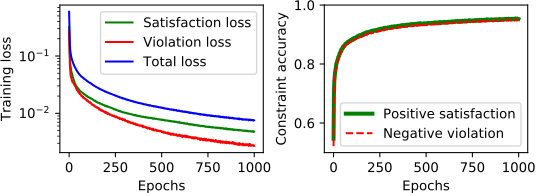
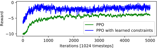
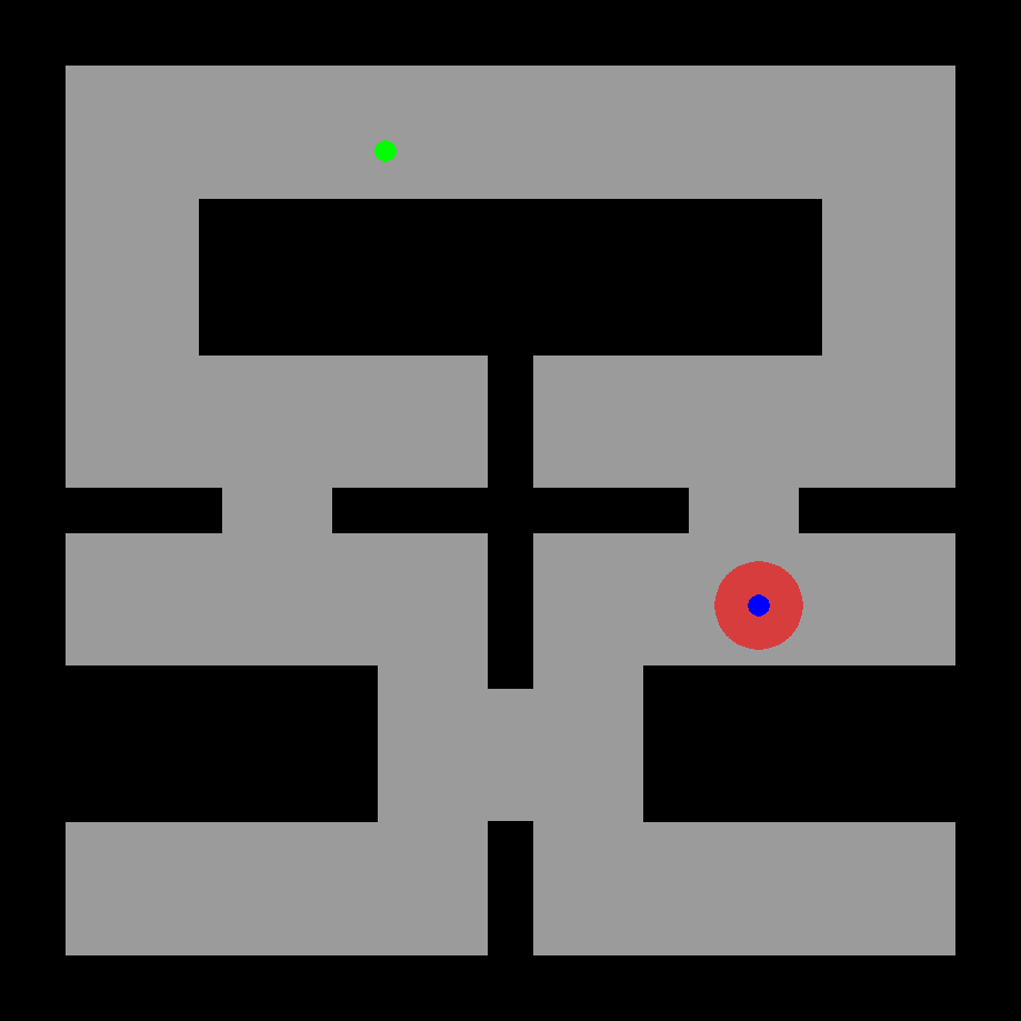
In a fixed two-dimensional maze, 500 mouse-controlled trajectories provide positive examples. Immediate failures and a task-specific reversed-path heuristic supply negatives, producing 7,228 positive and 15,994 negative pairs. A network learns two action inequalities from balanced minibatches. Classification accuracy improves with the loss, and using the constraints improves subsequent PPO rewards. These labeling shortcuts depend on the simple, effectively instantaneous position-control dynamics.
Refer to caption
Refer to caption
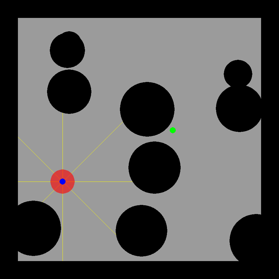
Figure 2: An agent (blue) is tasked to reach a target (green), while avoiding walls and obstacles (black) in a static maze (left) or with random obstacles (right) with shortest distances in eight directions (yellow). The agent can be controlled with position (within the red area) or force commands.
Original figure
(a) Loss and accuracy throughout constraint network training.
Original figure
(b) Reinforcement learning with and without learned constraints.
Figure 3: Minimizing the constraint loss indeed results in correct separation for good and negative demonstrations (a). After training, the learned constraints can guide exploration during reinforcement learning to achieve higher rewards (b).

4 Constrained Exploration and Recovery from Experience Shaping

4.1 Overview

For tasks with delayed consequences, the direct policy collects trajectories toward the goal. Actions followed by sufficiently long survival can be labeled positive, and terminal failure supplies a negative example. Actions near an unresolved ending remain uncertain. A chosen survival horizon sets the practical meaning of recoverability.

4.2 Demonstration Sorting by Learning Recovery

The recovery policy starts from uncertain successor states and is rewarded for surviving rather than completing the original task. Survival for the chosen horizon marks the preceding action as recoverable; repeated failed attempts mark it negative. Labels propagate along the tested trajectory, and checking near its midpoint reduces repeated trials. The method requires identifiable outcomes and the ability to restore selected states, or an adequate replay-based substitute.

4.3 Detailed Algorithm

The retained procedures alternate direct-policy sampling, recovery trials, replay-buffer updates, and constraint learning. The policy-gradient update stores the raw policy action, treating correction as part of environment interaction; the constraint learner stores the corrected action actually executed. Confusing these two actions would change the intended learning problem.

1: procedure CERES(ℰd,ℰr,𝒩dπ,𝒩rπ,𝒩C\mathcal{E}^{d},\mathcal{E}^{r},\mathcal{N}^{\pi}_{d},\mathcal{N}^{\pi}_{r},\mathcal{N}^{C})
2:   𝒩dπ\mathcal{N}^{\pi}_{d}.initialize(), 𝒩rπ\mathcal{N}^{\pi}_{r}.initialize(), 𝒩C\mathcal{N}^{C}.initialize()
3:   ℬ={}\mathcal{B}={\left\{{}\right\}} ⊳\triangleright Experience replay buffer start empty
4:   for iiter=1i_{\text{iter}}=1 to nitern_{\text{iter}} do
5:    τPOd,D+d,D−d,D∗d=Sample​(ℰd,𝒩dπ,𝒩C)\tau_{\text{PO}}^{d},D_{+}^{d},D_{-}^{d},D_{*}^{d}=\textsc{Sample}{{\left({\mathcal{E}^{d},\mathcal{N}^{\pi}_{d},\mathcal{N}^{C}}\right)}}
6:    UpdatePolicy​(𝒩dπ,τPOd)\textsc{UpdatePolicy}{{\left({\mathcal{N}^{\pi}_{d},\tau_{\text{PO}}^{d}}\right)}}
7:    τRLr,D+r,D−r,D∗r=Sample​(ℰr,𝒩rπ,𝒩C)\tau_{\text{RL}}^{r},D_{+}^{r},D_{-}^{r},D_{*}^{r}=\textsc{Sample}{{\left({\mathcal{E}^{r},\mathcal{N}^{\pi}_{r},\mathcal{N}^{C}}\right)}}
8:    UpdatePolicy​(𝒩rπ,τPOr)\textsc{UpdatePolicy}{{\left({\mathcal{N}^{\pi}_{r},\tau_{\text{PO}}^{r}}\right)}}
9:    ℬ\mathcal{B}.append(D+d,D−d,D+r,D−rD_{+}^{d},D_{-}^{d},D_{+}^{r},D_{-}^{r})
10:    UpdateConstraints​(𝒩C,ℬ)\textsc{UpdateConstraints}{{\left({\mathcal{N}^{C},\mathcal{B}}\right)}}
11:    ℰr\mathcal{E}^{r}.add_for_recovery(D∗d){{\left({D_{*}^{d}}\right)}}
12:   end for
13:   return trained 𝒩dπ,𝒩rπ,𝒩C\mathcal{N}^{\pi}_{d},\mathcal{N}^{\pi}_{r},\mathcal{N}^{C}
14: end procedure
Figure 4: In CERES, a direct control policy is trained together with a recovery policy, yielding positive and negative demonstrations to learn and apply action-space constraints.
1: procedure Sample(ℰ,𝒩π,𝒩C\mathcal{E},\mathcal{N}^{\pi},\mathcal{N}^{C})
2:   τPO=()\tau_{\text{PO}}=() ⊳\triangleright Trajectories for policy update
3:   τC=()\tau_{C}=() ⊳\triangleright Trajectories for demonstration evaluation
4:   𝐬=ℰ\mathbf{s}=\mathcal{E}.reset(); end=false\text{end}=\text{false} ⊳\triangleright Get initial state
5:   while not end do
6:    SS.add(𝐬\mathbf{s}) ⊳\triangleright Store current state
7:    𝐱=𝒩π​(𝐬)\mathbf{x}=\mathcal{N}^{\pi}(\mathbf{s}) ⊳\triangleright Predict action
8:    𝐆𝐬,𝐡𝐬=𝒩C​(𝐬)\mathbf{G}^{\mathbf{s}},\mathbf{h}^{\mathbf{s}}=\mathcal{N}^{C}(\mathbf{s}) ⊳\triangleright Predict constraints
9:    𝐱∗=Constrain​(𝐱,𝐆𝐬,𝐡𝐬)\mathbf{x}^{*}=\textsc{Constrain}{{\left({\mathbf{x},\mathbf{G}^{\mathbf{s}},\mathbf{h}^{\mathbf{s}}}\right)}} ⊳\triangleright Correct action
10:    𝐬~,r,end,info=ℰ.\widetilde{\mathbf{s}},r,\text{end},\text{info}=\mathcal{E}.do(𝐱∗){{\left({\mathbf{x}^{*}}\right)}} ⊳\triangleright Play corrected
11:    τPO\tau_{\text{PO}}.append(𝐬,𝐱,r,end){{\left({\mathbf{s},\mathbf{x},r,\text{end}}\right)}}
12:    τC\tau_{C}.append(𝐬,𝐱∗,info){{\left({\mathbf{s},\mathbf{x}^{*},\text{info}}\right)}}
13:   end while
14:   D+,D−,D∗=EvaluateDemos​(τC)D_{+},D_{-},D_{*}=\textsc{EvaluateDemos}{{\left({\tau_{C}}\right)}}
15:   return τPO,D+,D−,D∗\tau_{\text{PO}},D_{+},D_{-},D_{*}
16: end procedure
Figure 5: Trajectories are sampled for policy and constraint learning from positive, negative, uncertain demonstrations.

5 Experiments

5.1 Practical Implementation

Early constraint estimates can be inaccurate, so constraints are activated probabilistically according to their current classification accuracy. Some experiments constrain only the direct policy, allowing broader recovery exploration. This explicitly permits unconstrained and potentially unsafe actions during training.

5.2 Obstacle Avoidance with Dynamics

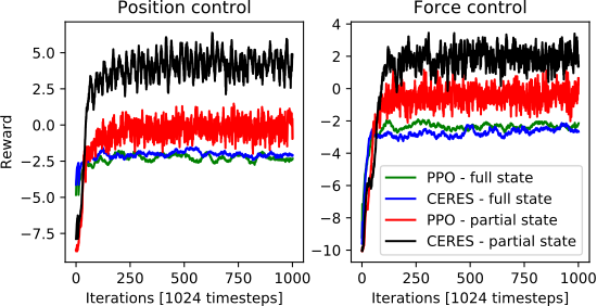
Random-obstacle experiments compare position increments with force control, where velocity and braking make safety depend on future steps. Four variants combine these action models with full or reduced observations for the main policy. In the reduced-observation condition, the constraint network still receives the full state, including eight obstacle-distance beams. CERES improves the reported reward curves relative to matched PPO runs; it delegates obstacle information to a separate network rather than eliminating the need to sense obstacles.
Original figure
Figure 6: Reinforcement learning on random obstacles.

6 Discussion and future work

Positive and negative experience can train useful action constraints, and recovery experiments extend the approach to delayed failures without initial expert demonstrations. The evidence is limited to simulated navigation, learned finite-horizon labels, and state-reset access. Transferring to real robots or tasks with ambiguous failure definitions remains future work; an inaccurate recovery policy can reject recoverable actions or fail to discover genuinely safe ones.

Concept demonstration

Open image ↗