Overview
This edition retains the complete paper’s seven numbered figures, four tables, two algorithms, and displayed equations. Subfigures remain paired with their original captions.
At a glance
IoU-Net predicts how well a detected bounding box overlaps its target, separating localization confidence from class confidence. The predicted overlap guides duplicate suppression and provides a differentiable objective for box refinement. On the reported MS-COCO validation split, a joint ResNet-101-FPN system improves average precision from 38.5 to 40.6. Gains concentrate at stricter overlap thresholds; low-overlap estimation error and additional computation remain limitations.
1 Introduction
Detection needs both the right label and an accurately placed box, but class scores do not directly measure localization. Ranking by class confidence can suppress a better box, and repeated regression can eventually worsen coordinates. IoU-Net adds a localization estimate that can rank boxes and guide gradient-based refinement. The contribution is compatible with the evaluated region-based detectors, rather than a new complete detection pipeline.
2 Delving into object localization
The diagnostic uses a standard feature-pyramid detector trained on COCO trainval35k and evaluated on minival. It separates errors caused by suppression from errors caused by repeated box regression.
2.1 Misaligned classification and localization accuracy
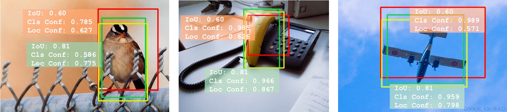
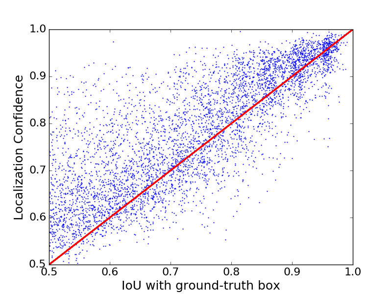
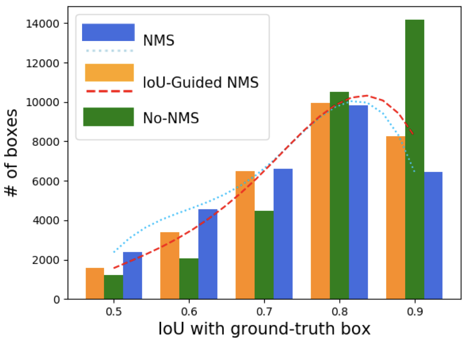
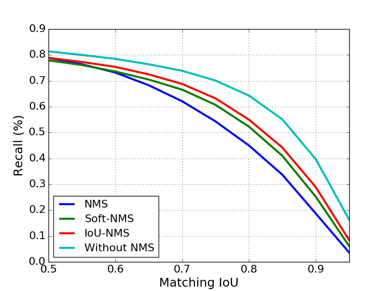
Class scores distinguish foreground from background under an overlap threshold; they are not trained to order every positive box by localization quality. For boxes above 0.5 overlap, the plotted correlation with class confidence is 0.217, compared with 0.617 for the learned localization estimate. Ordinary suppression removes many highly accurate boxes when a less accurate neighbor has a higher class score. The no-suppression reference measures available candidate recall, not a usable final detector with controlled duplicates.
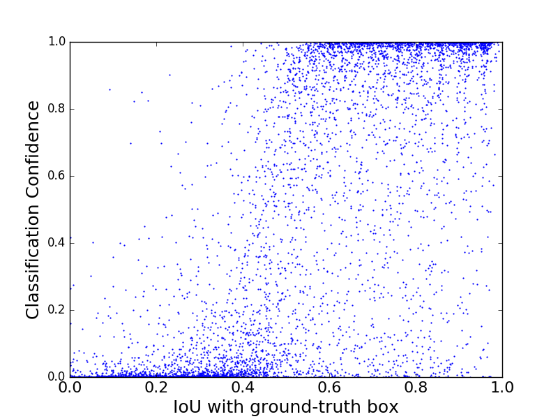
(a) The classification confidence indicates the category of a bounding box, but cannot be interpreted as the localization accuracy.
(b) To resolve the issue, we propose IoU-Net to predict the localization confidence for each detected bounding box, i.e., its IoU with corresponding ground-truth.
2.2 Non-monotonic bounding box regression
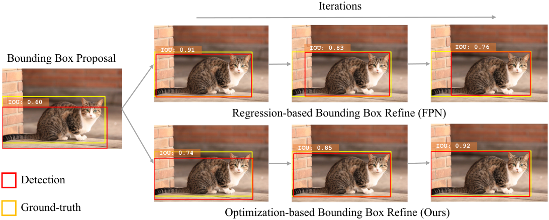
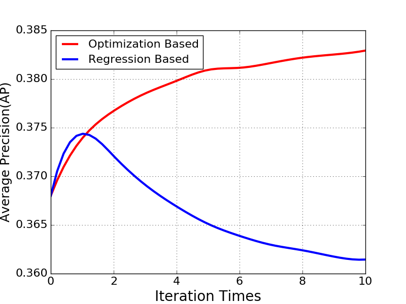
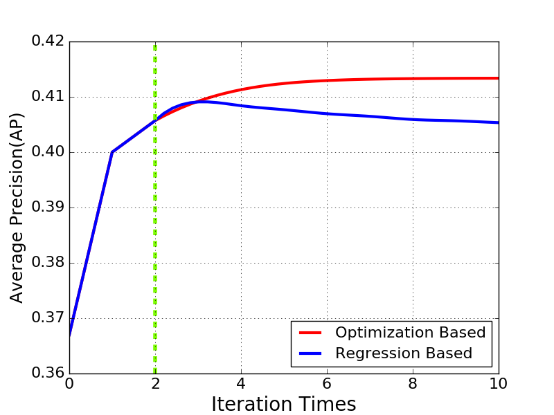
Bounding-box regression learns a transformation from proposals to targets. Feeding its output back repeatedly changes the input distribution and need not improve localization monotonically. Experiments with feature-pyramid and cascade detectors show precision dropping after sufficient repeated regression. A learned localization objective offers a stopping signal and a direction for refinement, although its quality still depends on prediction error.
3 IoU-Net
IoU-Net first learns an overlap predictor, then uses it for suppression and optimization-based refinement. The final experiment jointly trains this predictor alongside the detector.
3.1 Learning to predict IoU
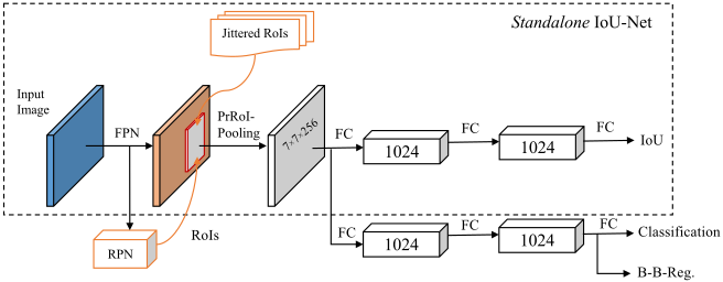
Training boxes are generated by randomly transforming ground-truth boxes rather than using only region proposals. Boxes below 0.5 overlap are discarded, and the remaining examples are sampled uniformly across overlap values. A class-aware two-layer head predicts overlap from pooled feature-pyramid features. This sampling is intended to reduce dependence on one detector’s proposal distribution; broad robustness beyond the tested detectors is not established.
3.2 IoU-guided NMS
IoU-guided suppression selects the remaining box with the highest predicted overlap, then suppresses sufficiently overlapping neighbors. The selected box inherits the maximum classification score among the boxes it suppresses. This keeps geometric ranking distinct from label confidence. Algorithm 1 preserves the complete procedure; inference uses predicted overlap, not ground-truth overlap.
is a set of detected bounding boxes.
and are functions (neural networks) mapping bounding boxes to their classification confidence and IoU estimation (localization confidence) respectively.
is the NMS threshold.
3.3 Bounding box refinement as an optimization procedure
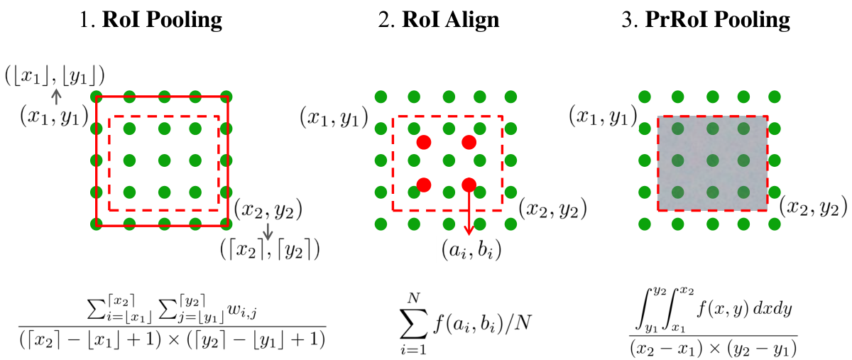
Refinement treats predicted IoU as an objective and performs gradient ascent on box coordinates, initialized by one ordinary regression step. Gradients are scaled by box dimensions, and stopping rules use predicted improvement and degeneration tolerance. Algorithm 2 and all equations are retained. Precise RoI Pooling integrates a bilinearly interpolated continuous feature map over each pooling bin, enabling continuous coordinate derivatives without quantization. The empirically monotonic improvements in the tested plots are not a general guarantee that optimizing estimated IoU always improves true overlap.
is a set of detected bounding boxes, in the form of .
is the feature map of the input image.
is number of steps. is the step size, and is an early-stop threshold and is an localization degeneration tolerance.
Function extracts the feature representation for a given bounding box and function denotes the estimation of IoU by the IoU-Net.
Equation 1
| (1) |
Equations 2–4
| (2) |
| (3) |
| (4) |
3.4 Joint training
The overlap head shares the ResNet-FPN backbone with classification and regression, with Precise RoI Pooling replacing ordinary pooling. It is trained with smooth-L1 loss on normalized overlap targets and separately generated boxes. Training uses 16-image batches for 160,000 iterations, with warmup and a learning-rate decrease after 120,000 steps. At inference, suppression runs first, followed by refinement of the 100 highest-class-confidence boxes. The reported refinement uses at most five iterations, step size 0.5, early-stop threshold 0.001, and degeneration tolerance -0.01.
4 Experiments
Experiments use the 80-category COCO detection benchmark: approximately 115,000 training images and 5,000 validation images. Standalone-predictor comparisons isolate suppression and refinement; the final experiments evaluate joint training. The preserved tables report both overall average precision and increasingly strict overlap thresholds.
4.1 IoU-guided NMS
IoU-guided suppression particularly improves strict-localization metrics. At matching overlap 0.9, recall is 18.7% after ordinary suppression and 28.9% after IoU-guided suppression, versus 39.7% before suppression. Overall gains are smaller and are not uniformly larger than Soft-NMS for every detector; for Cascade R-CNN, Table 1 gives 40.7 overall AP for IoU-NMS and 40.9 for Soft-NMS, while IoU-NMS has the higher AP90.
| Method | +Soft-NMS | +IoU-NMS | ||||||
|---|---|---|---|---|---|---|---|---|
| FPN | 36.4 | 58.0 | 53.1 | 44.9 | 31.2 | 9.8 | ||
| 36.8 | 57.5 | 53.1 | 45.7 | 32.3 | 10.3 | |||
| 37.3 | 56.0 | 52.2 | 45.6 | 33.9 | 13.3 | |||
| Cascade R-CNN | 40.6 | 59.3 | 55.2 | 49.1 | 38.7 | 16.7 | ||
| 40.9 | 58.2 | 54.7 | 49.4 | 39.9 | 17.8 | |||
| 40.7 | 58.0 | 54.7 | 49.2 | 38.8 | 18.9 | |||
| Mask-RCNN | 37.5 | 58.6 | 53.9 | 46.3 | 33.2 | 10.9 | ||
| 37.9 | 58.2 | 53.9 | 47.1 | 34.4 | 11.5 | |||
| 38.1 | 56.4 | 52.7 | 46.7 | 35.1 | 14.6 |
4.2 Optimization-based bounding box refinement
Adding optimization-based refinement improves the tested feature-pyramid, cascade, and mask detectors. For Cascade R-CNN, overall AP rises from 40.6 to 41.4 and AP90 from 16.7 to 19.5. These are increases of 0.8 and 2.8 percentage points, not relative percent gains.
| Method | +Refinement | ||||||
|---|---|---|---|---|---|---|---|
| FPN | 36.4 | 58.0 | 53.1 | 44.9 | 31.2 | 9.8 | |
| 38.0 | 57.7 | 53.1 | 46.1 | 34.3 | 14.6 | ||
| Cascade R-CNN | 40.6 | 59.3 | 55.2 | 49.1 | 38.7 | 16.7 | |
| 41.4 | 59.3 | 55.3 | 49.6 | 39.4 | 19.5 | ||
| Mask-RCNN | 37.5 | 58.6 | 53.9 | 46.3 | 33.2 | 10.9 | |
| 39.2 | 57.9 | 53.6 | 47.4 | 36.5 | 16.4 |
4.3 Joint training
Joint training plus suppression and refinement raises ResNet-50-FPN from 36.4 to 38.1 AP and ResNet-101-FPN from 38.5 to 40.6. On a TITAN X at 1200-by-800 input resolution, the listed ResNet-50 IoU-Net takes 0.305 seconds per image versus 0.255 for the FPN baseline. AP50 can decline because low-overlap boxes have more variable appearance and less accurate IoU estimates. Sampling more low-overlap training boxes is suggested as a partial remedy.
| Backbone | Method | +IoU-NMS | +Refine | ||||||
|---|---|---|---|---|---|---|---|---|---|
| ResNet-50 | FPN | 36.4 | 58.0 | 53.1 | 44.9 | 31.2 | 9.8 | ||
| IoU-Net | 37.0 | 58.3 | 53.8 | 45.7 | 31.9 | 10.7 | |||
| 37.6 | 56.2 | 52.4 | 46.0 | 34.1 | 14.0 | ||||
| 38.1 | 56.3 | 52.4 | 46.3 | 35.1 | 15.5 | ||||
| ResNet-101 | FPN | 38.5 | 60.3 | 55.5 | 47.6 | 33.8 | 11.3 | ||
| IoU-Net | 38.9 | 60.2 | 55.5 | 47.8 | 34.6 | 12.0 | |||
| 40.0 | 59.0 | 55.1 | 48.6 | 37.0 | 15.5 | ||||
| 40.6 | 59.0 | 55.2 | 49.0 | 38.0 | 17.1 |
| Method | FPN | Mask-RCNN | Cascade R-CNN | IoU-Net |
|---|---|---|---|---|
| Speed (sec./image) | 0.255 | 0.267 | 0.384 | 0.305 |
5 Conclusion
Localization confidence provides useful information that a class score alone omits. The experiments demonstrate improved high-overlap detection through separate geometric ranking and differentiable refinement. Benefits depend on the accuracy of the learned overlap predictor and add inference cost; the reported evidence is limited to the specified COCO split and detector families.