Behavioral cloning from observation (BCO) learns a policy from expert state sequences without the expert’s actions. Before seeing demonstrations, the agent explores to learn an inverse dynamics model; afterward it infers missing actions and clones them. Optional further interaction refines the model and policy. Experiments trade off demonstration data, task performance, and interaction before versus after demonstrations.
1 Introduction
Moving environment interaction before a demonstration becomes available can reduce the delay before imitating a new task. BCO learns how the agent’s own actions produce state changes, then reuses that knowledge to interpret demonstrations. “No post-demonstration interaction” does not mean no interaction overall: the initial dynamics-learning phase can be substantial.
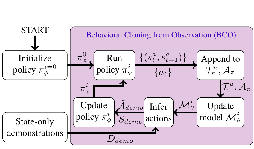
Figure 1: Behavioral Cloning from Observation (BCO()) framework proposed in this paper. The agent is initialized with a (random) policy which interacts with the environment and collects data to to learn its own agent-specific inverse dynamics model.
Then, given state-only demonstration information, the agent uses this learned model to infer the expert’s missing action information.
Once these actions have been inferred, the agent performs imitation learning. The updated policy is then used to collect data and this process repeats.
2 Related Work
Ordinary behavioral cloning requires action labels, while inverse reinforcement learning generally needs further environment interaction to optimize an inferred objective. BCO instead predicts actions from consecutive states using a learned inverse model. Its intended reusable component is the agent’s dynamics, rather than a reward tied to one task.
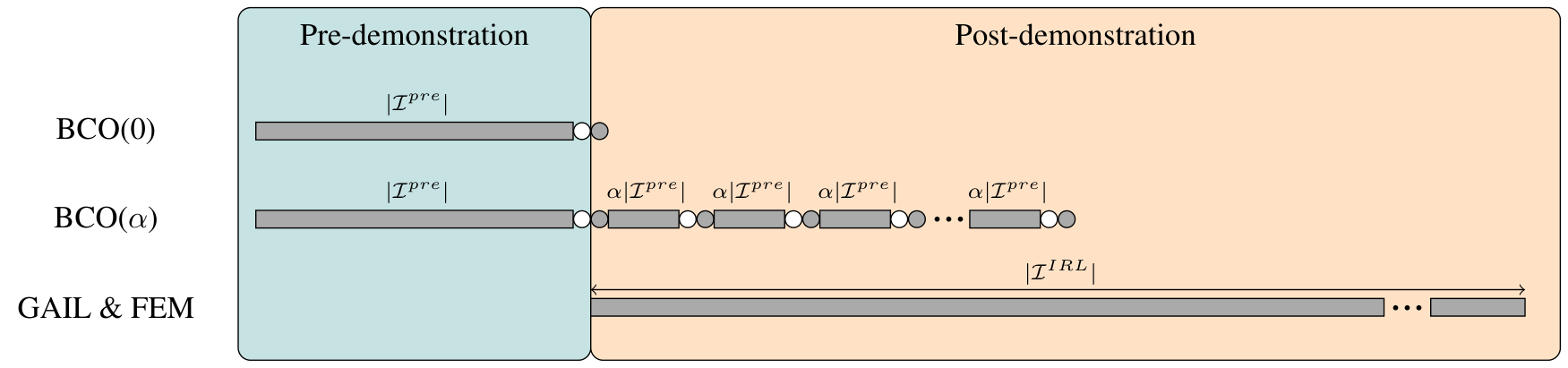
Figure 2: Learning timelines for BCO(), BCO(), and the IRL methods we compare against in this paper. The horizontal axis represents time, gray rectangles mark when each technique requires environment interactions. For BCO, the white and gray circles denote the inverse model and policy learning steps, respectively. For BCO, is the number of post-demonstration environment interactions performed before each model- and policy-improvement step and for IRL methods, represents the total number of interactions.
3 Problem Formulation
The setting assumes a Markov decision process and comparable demonstrated and learner state transitions. State features are partitioned into agent-specific and task-specific components; inverse dynamics uses the former, while the imitation policy can use the full state. The experiments use supplied state vectors, not raw tutorial videos or arbitrary human-to-robot embodiment transfer.
4 Behavioral Cloning from Observation
The retained algorithm first gathers exploratory transitions and fits inverse dynamics, then labels the observed expert transitions with inferred actions and trains a policy. Repeating these steps with data collected by the current imitation policy produces an optional refinement procedure.
4.1 Inverse Dynamics Model Learning
Random exploration supplies state-transition/action triples. Maximum-likelihood training maps consecutive agent states to an action distribution: categorical for discrete actions and Gaussian for continuous actions. The continuous model predicts action means with a neural network and learns state-independent standard deviations. Accuracy depends on whether exploration covers the transitions needed to interpret demonstrations.
Equation 1
(1)
4.2 Behavioral Cloning
The inverse model assigns the most likely action to each demonstrated state transition. Behavioral cloning then fits those inferred actions from the full demonstrated states. The policy therefore inherits errors from action inference as well as the usual distribution shift of supervised imitation.
10:
Generate set of agent-specific state transitions from the demonstrated state trajectories
11:
Use with to approximate
12:
Improve by behavioralCloning()
13:
Set
14:endwhile
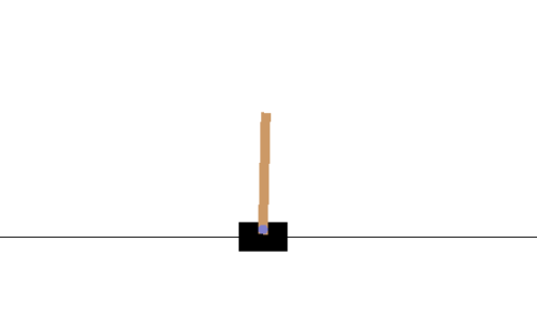
(a)CartPole
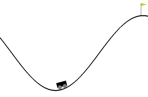
(b)MountainCar
(c)Reacher
(d)Ant
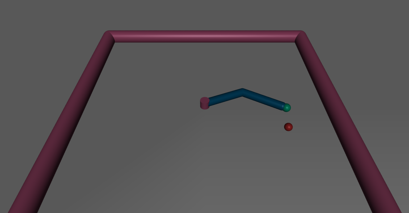
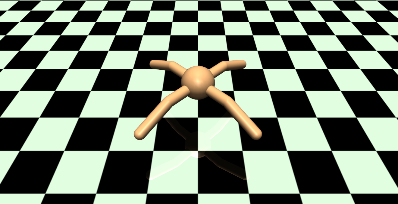
Figure 3: Representative screenshots of the domains considered in this paper.
4.3 Model Improvement
BCO(α) executes its current policy, updates inverse dynamics from the new transitions, and refits the imitation policy. Each round uses α times the initial exploration budget; after T rounds, the extra interaction budget is Tα times that initial budget. BCO(0) skips this refinement. Larger α can improve performance while increasing post-demonstration cost.
5 Implementation and Experimental Results
Tests use CartPole, MountainCar, Reacher, and Ant simulations, with experts trained by trust region policy optimization (TRPO). Comparisons include behavioral cloning, feature expectation matching (FEM), and generative adversarial imitation learning (GAIL). BCO alone lacks expert action labels, but has its own pre-demonstration exploration data; methods therefore have different information and interaction budgets.
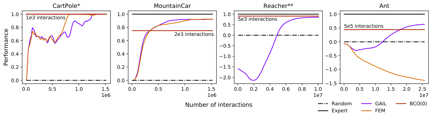
Figure 4: Performance of each technique with respect to the number of post-demonstration interactions. For each domain, ten demonstrated trajectories were considered. BCO(0) is depicted as a horizontal line since all environment interactions happen before the demonstration is provided. Performance values are scaled such that performance of a random policy is zero and the performance of the expert is one. Note that GAIL and FEM have access to demonstration action information whereas BCO does not. *The BCO line is not visible for the CartPole domain because BCO has the same performance as the expert. **FEM is not shown for the Reacher domain because its performance is much worse than the other techniques.
.
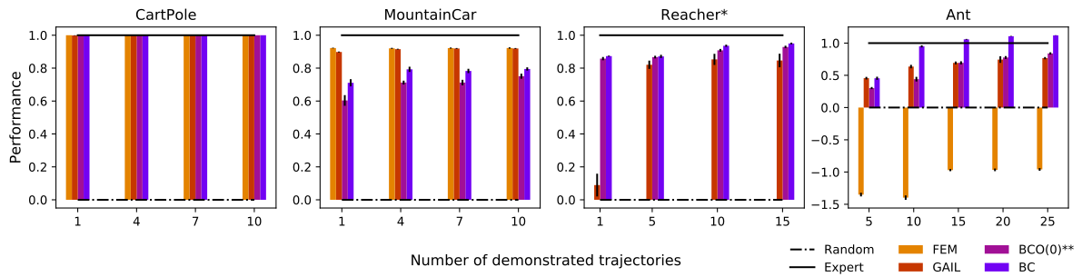
Figure 5: Performance of imitation agents with respect to the number of available demonstration trajectories. Rectangular bars and error bars represent the mean return and the standard error, respectively, as measured over 5000 trajectories. Returns have been scaled such that the performance of a random policy and the demonstrating agent are zero and one, respectively. *Note that FEM is not shown for the Reacher domain because its performance is much worse than the others.
**Note that BC, GAIL, and FEM all have access to demonstration action information whereas BCO(0) does not.
5.1 Training Details and Results
Initial inverse-model data comprise 1,000 interactions for CartPole, 2,000 for MountainCar, 5,000 for Reacher, and 500,000 for Ant. Models range from linear functions to two-layer networks. Reacher separates arm state from target position to reuse dynamics across targets. BCO and behavioral cloning reserve 30% of their data for validation and stop when validation error rises; other methods use all available training data.
5.2 Discussion
Results average twenty runs. In the plotted comparison, GAIL and FEM require at least forty times as many interactions to reach the BCO(0) performance level, while BCO’s exploration happens before demonstrations. This supports reduced post-demonstration delay rather than interaction-free learning. Final normalized returns average 5,000 evaluation episodes, with random and expert performance scaled to zero and one. BCO is weaker on MountainCar, competitive on Reacher and Ant, and improves with additional model-refinement interaction. Coverage, model error, and dependence on state observations limit generalization beyond these simulations.
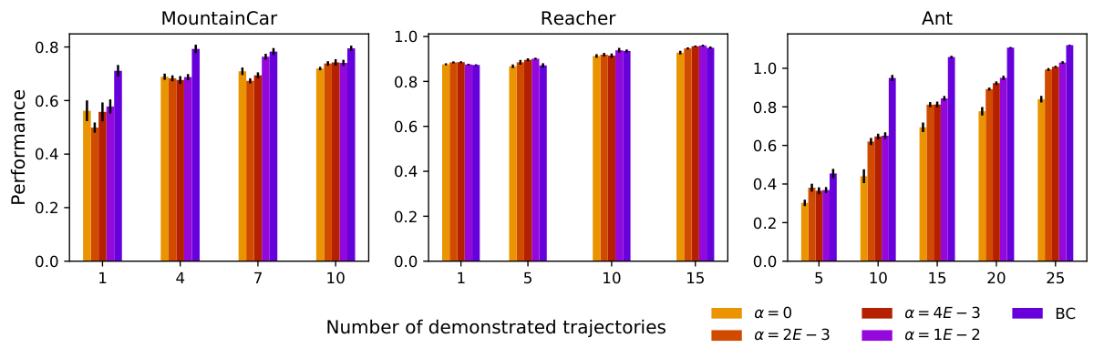
Figure 6: The performance of BC and several BCO() techniques (varying ) with respect to the number of demonstrated trajectories provided. Rectangular bars and error bars represent the mean return and the standard error, respectively, as measured over 5000 trajectories. By increasing , more post-demonstration environment interactions are allowed to occur, which increases the performance of the imitation policy. Note that BC has access to demonstration action information whereas BCO does not. Also note that the number of trajectories required for learning a fairly good policy is very small. Each demonstrated trajectory has 5, 50, and 50 transitions for each domain from left to right, respectively. Note that we did not demonstrate the results for CartPole because the results were equally perfect regardless of the value of .
MountainCar (pre-demo )
Reacher (pre-demo )
Ant (pre-demo )
Table 1: This is an extension to Figure 6 which provides the number of post-demonstration interactions for each case. First vertical column for each domain () shows the number of demonstrated trajectories. As an example, for the MountainCar domain with demonstrated trajectory and , the average number of post-demonstration interactions is 6825. We can also see at the top of the table that the number of pre-demonstration interactions is so the overall number of interactions would become . It can be seen that almost always by increasing or the number of demonstrated trajectories, the number of post-demonstration interactions increases. Also the overall number of interactions (combined pre- and post-demonstration interactions) in all the cases is far less than the overall number of interactions required by the other methods (FEM and GAIL).
6 Conclusions
A reusable inverse dynamics model can turn state-only demonstrations into supervised policy targets and enable imitation without additional post-demonstration interaction. Optional refinement improves the performance–interaction tradeoff, but prior exploration and compatible state representations remain necessary.
Acknowledgments
The authors disclose Peter Stone’s service on Cogitai’s board and the university’s review of that arrangement.
23 references
Argall et al. [2009]
Brenna D Argall, Sonia Chernova, Manuela Veloso, and Brett Browning.
A survey of robot learning from demonstration.
Robotics and autonomous systems, 57(5):469–483, 2009.
Bojarski et al. [2016]
Mariusz Bojarski, Davide Del Testa, Daniel Dworakowski, Bernhard Firner, Beat
Flepp, Prasoon Goyal, Lawrence D Jackel, Mathew Monfort, Urs Muller, Jiakai
Zhang, et al.
End to end learning for self-driving cars.
arXiv preprint arXiv:1604.07316, 2016.
Brockman et al. [2016]
Greg Brockman, Vicki Cheung, Ludwig Pettersson, Jonas Schneider, John Schulman,
Jie Tang, and Wojciech Zaremba.
OpenAI Gym.
arXiv preprint arXiv:1606.01540, 2016.
Chebotar et al. [2017]
Yevgen Chebotar, Karol Hausman, Marvin Zhang, Gaurav Sukhatme, Stefan Schaal,
and Sergey Levine.
Combining model-based and model-free updates for trajectory-centric
reinforcement learning.
arXiv preprint arXiv:1703.03078, 2017.
Daftry et al. [2016]
Shreyansh Daftry, J Andrew Bagnell, and Martial Hebert.
Learning transferable policies for monocular reactive mav control.
In International Symposium on Experimental Robotics, pages
3–11. Springer, 2016.
Finn et al. [2016]
Chelsea Finn, Sergey Levine, and Pieter Abbeel.
Guided cost learning: Deep inverse optimal control via policy
optimization.
In International Conference on Machine Learning, pages 49–58,
2016.
Giusti et al. [2016]
Alessandro Giusti, Jérôme Guzzi, Dan C Cireşan, Fang-Lin He,
Juan P Rodríguez, Flavio Fontana, Matthias Faessler, Christian Forster,
Jürgen Schmidhuber, Gianni Di Caro, et al.
A machine learning approach to visual perception of forest trails for
mobile robots.
IEEE Robotics and Automation Letters, 1(2):661–667, 2016.
Hanna and Stone [2017]
Josiah P Hanna and Peter Stone.
Grounded action transformation for robot learning in simulation.
In AAAI, pages 3834–3840, 2017.
Ho and Ermon [2016]
Jonathan Ho and Stefano Ermon.
Generative adversarial imitation learning.
In Advances in Neural Information Processing Systems, pages
4565–4573, 2016.
Ho et al. [2016]
Jonathan Ho, Jayesh Gupta, and Stefano Ermon.
Model-free imitation learning with policy optimization.
In International Conference on Machine Learning, pages
2760–2769, 2016.
Konidaris [2006]
George D Konidaris.
A framework for transfer in reinforcement learning.
In ICML-06 Workshop on Structural Knowledge Transfer for Machine
Learning, 2006.
Liu et al. [2017]
YuXuan Liu, Abhishek Gupta, Pieter Abbeel, and Sergey Levine.
Imitation from observation: Learning to imitate behaviors from raw
video via context translation.
arXiv preprint arXiv:1707.03374, 2017.
Niekum et al. [2015]
Scott Niekum, Sarah Osentoski, George Konidaris, Sachin Chitta, Bhaskara
Marthi, and Andrew G Barto.
Learning grounded finite-state representations from unstructured
demonstrations.
The International Journal of Robotics Research, 34(2):131–157,
2015.
Ross and Bagnell [2010]
Stéphane Ross and Drew Bagnell.
Efficient reductions for imitation learning.
In Proceedings of the thirteenth international conference on
artificial intelligence and statistics, pages 661–668, 2010.
Ross et al. [2011]
Stéphane Ross, Geoffrey J Gordon, and Drew Bagnell.
A reduction of imitation learning and structured prediction to
no-regret online learning.
In International Conference on Artificial Intelligence and
Statistics, pages 627–635, 2011.
Schulman et al. [2015]
John Schulman, Sergey Levine, Pieter Abbeel, Michael Jordan, and Philipp
Moritz.
Trust region policy optimization.
In Proceedings of the 32nd International Conference on Machine
Learning (ICML-15), pages 1889–1897, 2015.
Taylor et al. [2008]
Matthew E Taylor, Nicholas K Jong, and Peter Stone.
Transferring instances for model-based reinforcement learning.
In Joint European Conference on Machine Learning and Knowledge
Discovery in Databases, pages 488–505. Springer, 2008.
Todorov et al. [2012]
Emanuel Todorov, Tom Erez, and Yuval Tassa.
Mujoco: A physics engine for model-based control.
In Intelligent Robots and Systems (IROS), 2012 IEEE/RSJ
International Conference on, pages 5026–5033. IEEE, 2012.