At a glance
CVF learns smooth autonomous vector fields from demonstrations using matrix-valued kernels, prescribed equilibria, and convex constraints on the Jacobian. Random features make fitting and rollout faster. Curl-free kernels additionally yield gradient flows of learned potentials. Handwriting benchmarks show competitive accuracy and recovery, but the fitted contraction constraints are sampled locally rather than a global certificate over all states.
I Introduction
Fitting observed velocities alone can produce divergent rollouts from slightly different initial conditions. The proposed approach controls the geometry of the learned field around demonstrations, seeking a region in which neighboring trajectories draw together and recover toward the demonstrated behavior. Desired equilibrium locations are enforced exactly by construction.
Equation
I-A Preview
The objective combines squared velocity error and RKHS regularization. Linear matrix inequalities constrain the symmetric Jacobian at selected points. A modified kernel makes every candidate field vanish at the chosen equilibria, while a representer theorem converts functional optimization to a finite convex problem. Random-feature approximations reduce its size and evaluation cost.
Equations 1–2
| (1) | |||||
| (2) |
II Background: Stability of Dynamical Systems
The paper distinguishes convergence to an equilibrium from convergence between neighboring trajectories, then relates these properties to existing imitation methods.
II-A Notions of Stability and Lyapunov Analysis
A Lyapunov function decreases along a trajectory and can certify local or global asymptotic stability under the appropriate positivity and domain conditions. Finding such a function for general nonlinear dynamics is difficult. Linear systems and some polynomial systems admit specialized searches, but these do not cover every stable nonlinear system.
Equation 3
| (3) |
II-B Incremental Stability and Contraction Analysis
Contraction concerns the separation between trajectories. A uniformly negative symmetric Jacobian in a suitable invariant region makes infinitesimal Euclidean distances shrink exponentially. If contraction holds throughout the state space and an equilibrium exists, that equilibrium is unique and globally attracting. A more general state-dependent metric can certify contraction when the Euclidean test fails. [18]
The learning formulation enforces inequalities at finitely many samples. Smoothness may extend the behavior around those samples, but sampled constraints alone do not certify every point in the surrounding region or the entire state space.
Equations 4
| (4) |
II-C Prior Work in Learning Stable Dynamical Systems
DMPs combine a phase-dependent nonlinear motion component with an attracting linear system. SEDS constrains a Gaussian-mixture field using a fixed quadratic Lyapunov function. CLF-DM fits a more flexible potential and uses it to stabilize a regression model. The latter two involve nonconvex fitting; CVF instead solves a convex constrained regression problem for fixed features and hyperparameters. [11], [14], [15]
III Learning Contracting Vector Fields
Vector-valued RKHS methods provide a smooth, regularized function class with direct control of field values and derivatives.
III-A Vector Fields generated by Matrix-valued Kernels
A matrix-valued kernel couples the output components of the vector field. The reproducing property makes point evaluation continuous and yields finite representations for regularized learning. Because contraction constraints depend on derivatives, an extended representer theorem includes both kernel sections and their derivatives. The resulting finite optimization has linear matrix inequalities in its coefficients.
Equations 5–7
| (5) |
| (6) |
| (7) |
III-B Choice of Matrix-valued Kernels
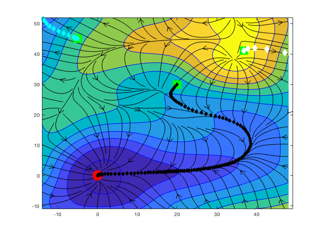
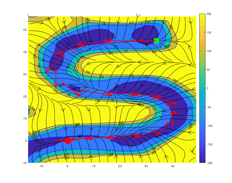
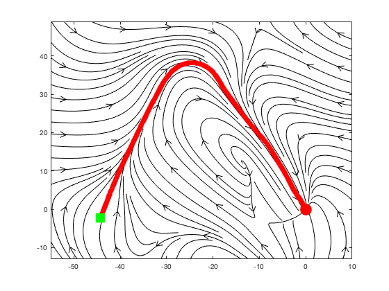
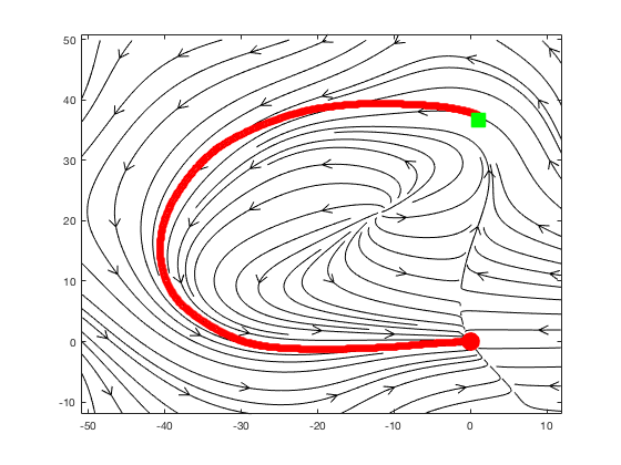
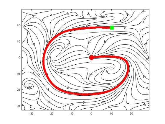
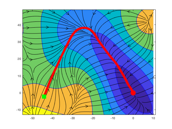
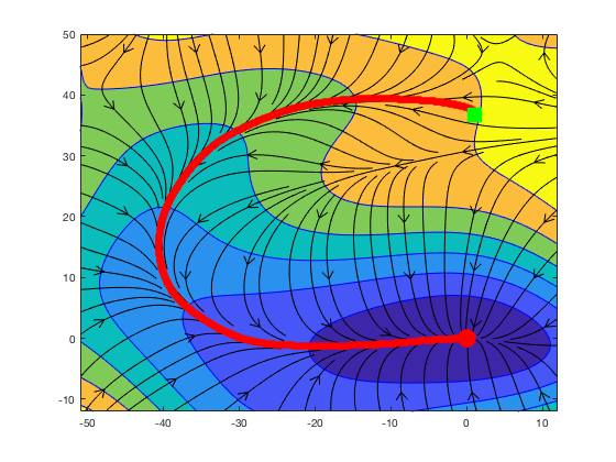
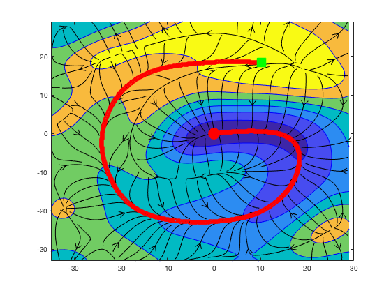
The Gaussian separable kernel gives each velocity component an ordinary Gaussian-kernel model. The curl-free kernel, obtained from Gaussian derivatives, instead constrains the field to be a gradient flow. It therefore admits a potential and a symmetric Jacobian. These choices impose different geometric biases, visible in the learned streamlines and potential contours.
Equations 8–10
| (8) |
| (9) |
| (10) |
III-C Subspace of RKHS Vector Fields that Vanish on a Point Set
Subtracting the kernel’s projection onto evaluations at the prescribed equilibrium set produces a new kernel that vanishes there. Every field in the corresponding subspace therefore has exactly zero velocity at those locations. This enforces the requested equilibria, without claiming that no other equilibria can exist outside a certified contraction region.
Equations 11
| (11) |
III-D Faster Solutions using Random Feature Approximations
The full kernel expansion grows with demonstration count and state dimension, making both training and numerical integration expensive. A low-rank matrix feature map replaces the expansion with a fixed-dimensional parameter vector. Feature count trades approximation quality against optimization and inference cost.
Equations
III-D 1 Matrix-valued Random Feature Maps for Gaussian Separable and Curl-free Kernels
Random Fourier features approximate the Gaussian separable kernel. Differentiated sinusoidal features yield a corresponding curl-free construction. The retained formulas specify the frequency distribution, phases, Kronecker structure, and feature scaling.
Equations 12–14
| (12) |
| (13) | |||||
| (14) |
III-D 2 Random Features Vanishing on a Point Set
An orthogonal projection removes the feature directions that produce nonzero values at the desired equilibria. This preserves exact zeros even though the base kernel is only approximated. The resulting kernel need not remain shift invariant.
Equations 15
| (15) |
III-E Regression with LMI Constraints
The finite model is linear in its coefficients, so squared-error fitting with coefficient regularization and sampled Jacobian inequalities remains convex. The implementation uses the SCS conic solver with an ADMM-based first-order method and direct linear solves. Constraints can be imposed on a subset of points; slack variables can relax infeasible specifications.
Equations 16–18
| (16) |
| (17) | |||||
| (18) |
IV Empirical Analysis
Experiments evaluate reproduction, convergence from unfamiliar starts, and computational scaling. The main comparison uses four planar handwriting shapes.
IV-A Imitating Human Handwriting Motions
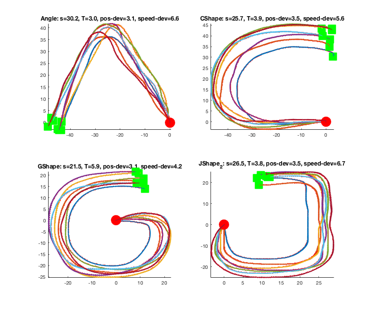
LASA contains thirty motions with seven demonstrations each and one thousand position–velocity samples per demonstration. The quantitative comparison selects Angle, CShape, GShape, and JShape. Four demonstrations train each model and three are held out; CVF and DMP train on the average training trajectory.
.
IV-B Qualitative Results
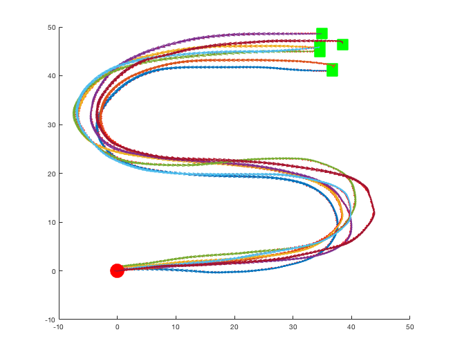
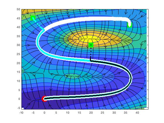
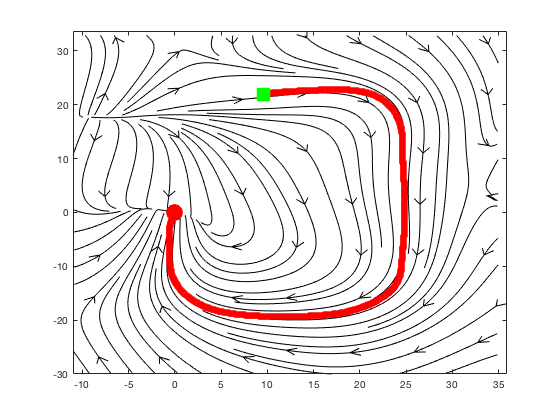
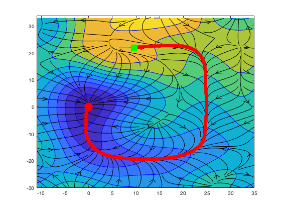
Plots show the largest symmetric-Jacobian eigenvalue around an S-shaped demonstration and compare separable and curl-free fields on other shapes. Both can form sizeable local contraction regions. The curl-free model also exposes a learned potential. These visualizations illustrate local geometry rather than establish a global convergence certificate.
IV-C Comparison Metrics
Trajectory and velocity errors measure reproduction over the demonstrated duration. Goal distance, time to enter a one-millimeter goal ball, and success over a horizon thirty times longer distinguish accurate paths from slow convergence. Sixteen grid starts per shape test broader recovery; DTW compares their paths with demonstrations. Training and integration times measure computational cost.
Equations 19–20
| (19) | |||
| (20) |
IV-D Comparison with DMP, SEDS and CLFDM
CVF-CF and CVF-GS use 100 or 200 random features, bandwidth 5 or 10, and contraction constraints at 250 points. Crucially, the quantitative comparison sets the contraction margin τ to zero; the separate S-shaped visualization uses a positive margin. Thus the benchmark constraints impose nonexpansion at samples rather than strict contraction everywhere.
Across the four shapes, CVF is among the two lowest mean trajectory errors on three and gives the best mean grid-start DTW on all four. The authors report one failed convergence case among the tested CVF starts. Training can cost more than the baselines, while inference remains comparable; looser solver stopping criteria reduce fitting cost. The four original tables retain all metrics and method-specific tradeoffs.
| DMP | SEDS | CLFDM | |
|---|---|---|---|
| TrainingTrajectoryError | 4.10 | 7.18 | 4.93 |
| TrainingVelocityError | 7.40 | 14.62 | 10.99 |
| TestTrajectoryError | 5.53 | 4.58 | 12.24 |
| TestVelocityError | 8.74 | 11.43 | 15.50 |
| DistanceToGoal | 3.59 | 3.25 | 6.70 |
| DurationToGoal | - | 3.89 | 4.34 |
| NumberReachedGoal | 0.00 | 7.00 | 7.00 |
| GridDuration | 5.91 | 3.72 | 9.73 |
| GridFractionReachedGoal | 0.06 | 1.00 | 1.00 |
| GridDistanceToGoal | 3.33 | 1.00 | 1.00 |
| GridDTWD | 24493.27 | 13865.75 | 14503.13 |
| TrainingTime | 0.05 | 2.10 | 2.82 |
| IntegrationSpeed | 0.21 | 0.06 | 0.15 |
| DMP | SEDS | CLFDM | |
|---|---|---|---|
| TrainingTrajectoryError | 4.40 | 8.29 | 6.90 |
| TrainingVelocityError | 7.32 | 14.73 | 12.65 |
| TestTrajectoryError | 6.99 | 9.08 | 5.82 |
| TestVelocityError | 9.43 | 12.59 | 10.89 |
| DistanceToGoal | 3.76 | 1.30 | 1.92 |
| DurationToGoal | - | 3.71 | 3.39 |
| NumberReachedGoal | 0.00 | 7.00 | 2.00 |
| GridDuration | - | 2.08 | 1.40 |
| GridFractionReachedGoal | 0.00 | 1.0 | 0.38 |
| GridDistanceToGoal | 3.96 | 1.0 | 2.22 |
| GridDTWD | 25679.59 | 14652 | 121312.43 |
| TrainingTime | 0.02 | 5.34 | 6.11 |
| IntegrationSpeed | 0.21 | 0.03 | 0.04 |
| DMP | SEDS | CLFDM | |
|---|---|---|---|
| TrainingTrajectoryError | 3.81 | 7.84 | 6.41 |
| TrainingVelocityError | 5.85 | 12.12 | 9.83 |
| TestTrajectoryError | 5.56 | 10.44 | 11.00 |
| TestVelocityError | 7.04 | 14.84 | 16.07 |
| DistanceToGoal | 1.63 | 0.18 | 3.72 |
| DurationToGoal | - | 4.86 | 15.08 |
| NumberReachedGoal | 0.00 | 7.00 | 7.00 |
| GridDuration | - | 2.78 | 12.68 |
| GridFractionReachedGoal | 0.00 | 1.00 | 1.00 |
| GridDistanceToGoal | 1.71 | 1.00 | 1.00 |
| GridDTWD | 19085.48 | 11493 | 10928.89 |
| TrainingTime | 0.02 | 14.43 | 3.01 |
| IntegrationSpeed | 0.18 | 0.08 | 0.10 |
| DMP | SEDS | CLFDM | |
|---|---|---|---|
| TrainingTrajectoryError | 3.09 | 14.37 | 4.96 |
| TrainingVelocityError | 6.05 | 22.88 | 9.60 |
| TestTrajectoryError | 5.47 | 16.85 | 4.95 |
| TestVelocityError | 8.49 | 25.76 | 9.81 |
| DistanceToGoal | 2.24 | 0.00 | 6.07 |
| DurationToGoal | - | 2.05 | 3.49 |
| NumberReachedGoal | 0.00 | 7.00 | 5.00 |
| GridDuration | 100.73 | 1.21 | 2.18 |
| GridFractionReachedGoal | 0.44 | 1.00 | 0.69 |
| GridDistanceToGoal | 1.42 | 1.00 | 3.61 |
| GridDTWD | 29568.10 | 12866 | 15403.52 |
| TrainingTime | 0.01 | 18.15 | 2.66 |
| IntegrationSpeed | 0.19 | 0.11 | 0.09 |
IV-E Scalability wrt Dimensions and Random Features
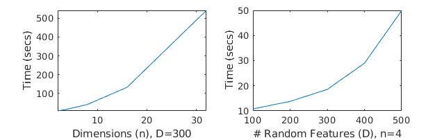
A planar S trajectory is embedded in dimensions 2, 4, 8, 16, and 32 with 300 curl-free features. A second sweep fixes dimension four and varies feature count from 100 to 500. With 6,000 SCS iterations, the reported residuals and gaps are approximately 10⁻⁶–10⁻⁴. Training scales roughly linearly with feature count and superlinearly with dimension in these tests; embedding planar data is not equivalent to learning arbitrary high-dimensional robot behavior.
IV-F Conclusion
The framework combines kernel regression, exact equilibrium placement, sampled contraction conditions, and convex optimization. Promising extensions include learned contraction metrics, modular composition, obstacle avoidance, and perception. The evidence here is handwriting simulation, with no physical-robot or global state-space safety evaluation.