Literature
Display
← All papers

Shampoo: Preconditioned Stochastic Tensor Optimization

Vineet Gupta · Tomer Koren † † footnotemark: · Yoram Singer

· ICML 2018, Proceedings of Machine Learning Research 80:1842–1850 ↗

Optimization9 min text · CondensedOriginal paper ↗
Contents

At a glance

Intuition. A preconditioner adjusts a proposed gradient step using past gradients, reducing repeated overshooting along strongly scaled directions. Shampoo remembers how rows and columns move together instead of treating every matrix entry as an unrelated knob. For a 2×3 weight matrix, its two preconditioners contain 4+9 entries; a full preconditioner over all six weights contains 36.

Reading the math. G is the current gradient matrix; L accumulates GGᵀ and R accumulates GᵀG, with small positive diagonal terms for stability. The update L⁻¼ G R⁻¼ rescales the gradient from both sides. Matrix powers act on eigenvalues, so the rescaling can follow tilted directions as well as coordinate axes.

Shampoo preconditions matrix and tensor gradients using one accumulated second-moment matrix per tensor dimension. It retains correlations within those dimensions while avoiding a full preconditioner over every flattened parameter. The paper proves rank-dependent regret bounds for online convex optimization and reports faster progress per training step in several neural-network experiments. Those experiments use nonconvex models and practical modifications; they are separate evidence from the convex theorem. Complete figures, algorithms, mathematical displays, and all fifteen formal statements are retained.

1 Introduction

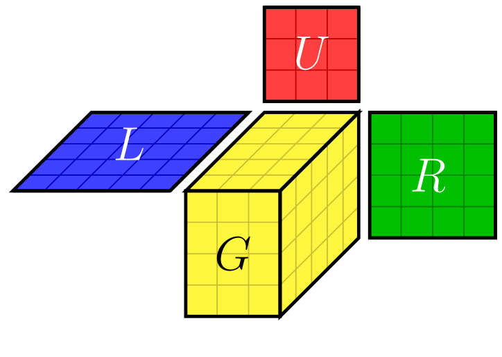
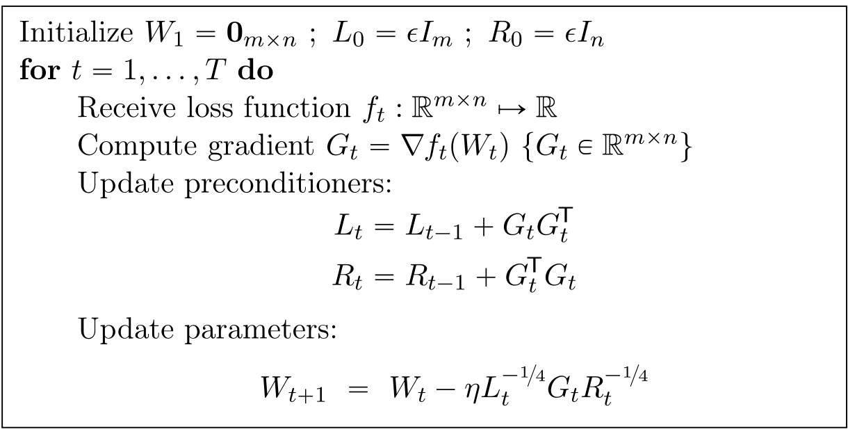
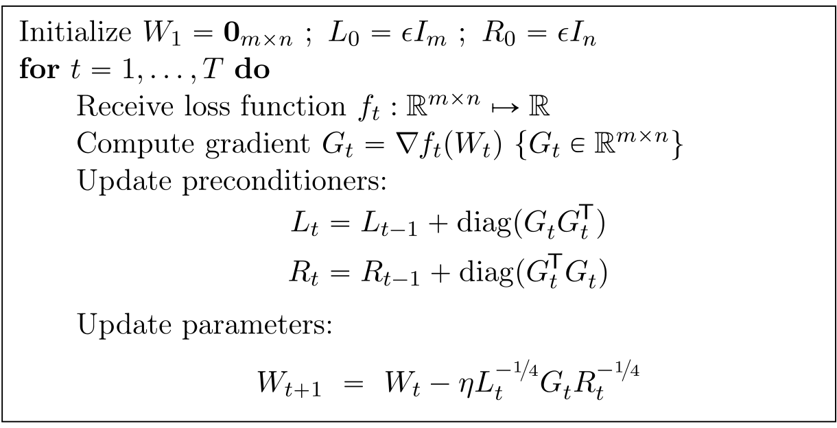
A full preconditioner for a flattened tensor can be too large to store or factor. Shampoo instead exploits the tensor’s existing shape, building modest matrices along each mode. Figure 1 illustrates the idea, and Algorithm 1 gives the matrix case. This is a structured second-moment method, not direct computation of a neural network’s Hessian or Fisher inverse. Its theoretical development uses online convex optimization, while its practical motivation includes deep learning.

Complete original S1.F1 from the exact-version PDF, including every panel, label, and original color.
Figure 1: Illustration of Shampoo for a 33-dimensional tensor G∈ℝ3×4×5G\in\mathbb{R}^{3\times 4\times 5}.
Complete original alg1 from the exact-version PDF, including every panel, label, and original color.
Algorithm 1: Shampoo, matrix case.
Accessible original algorithm markup

 Initialize W1=𝟎m×n;L0=ϵ​Im;R0=ϵ​InW_{1}=\bm{0}_{m\times n}~;~L_{0}=\epsilon I_{m}~;~R_{0}=\epsilon I_{n}  for t=1,…,Tt=1,\ldots,T do   Receive loss function ft:ℝm×n↦ℝf_{t}:\mathbb{R}^{m\times n}\mapsto\mathbb{R}   Compute gradient Gt=∇ft​(Wt)G_{t}=\nabla\mkern-1.0muf_{t}(W_{t}) {Gt∈ℝm×nG_{t}\in\mathbb{R}^{m\times n}}   Update preconditioners:

Equation Lt\displaystyle L_{t} =Lt−1+Gt​Gt𝖳\displaystyle=L_{t-1}+G_{t}G_{t}^{\mkern-1.5mu\scriptstyle\mathsf{T}} Rt\displaystyle R_{t} =Rt−1+Gt𝖳​Gt\displaystyle=R_{t-1}+G_{t}^{\mkern-1.5mu\scriptstyle\mathsf{T}}G_{t}
  Update parameters:
EquationWt+1=Wt−η​Lt−1/4​Gt​Rt−1/4W_{t+1}~=~W_{t}-\eta L_{t}^{-\nicefrac{{1}}{{4}}}G_{t}R_{t}^{-\nicefrac{{1}}{{4}}}

1.1 Shampoo for matrices

For an m×n parameter matrix, Shampoo accumulates left and right gradient Gram matrices, then multiplies the gradient by their inverse fourth roots. Storage for the preconditioners is m²+n² rather than m²n²; dense factorization costs scale as m³+n³ rather than m³n³. Tensor shape therefore matters. The equivalent flattened update uses a Kronecker-product metric without forming it explicitly. The fourth-root exponents are essential: replacing them with arbitrary inverse powers changes both the update and the analysis.

1.2 Related work

The method is closely related to full-matrix AdaGrad [6], but uses a structured implicit preconditioner instead of a dense matrix or an entirely elementwise approximation. K-FAC also uses Kronecker factors, but approximates a generative model’s Fisher matrix using network-specific gradient structure and statistical assumptions. Shampoo uses ordinary gradients and tensor dimensions in a more general optimization setting. Shared factorization ideas do not make these algorithms mathematically identical.

2 Background and technical tools

The analysis uses positive-semidefinite ordering, matrix powers defined spectrally, metric-induced norms, spectral norms, and Frobenius inner products. Negative matrix powers require positive-definite regularization or an explicitly defined generalized-inverse convention; a singular PSD matrix does not have an ordinary inverse. The preserved source definitions should be interpreted with that domain restriction.

2.1 Online convex optimization

In online convex optimization, the learner chooses an iterate, receives a convex loss, and competes with one fixed comparator over the full sequence. Regret measures the cumulative difference. Online-to-batch conversion gives stochastic convex optimization guarantees under the corresponding sampling and averaging setup. This framework does not directly prove convergence to a global minimum for the neural experiments.

Equation
ℛT=∑t=1Tft​(wt)−min⁡∑t=1Tw∈𝒲⁡ft​(w),\displaystyle\mathcal{R}_{T}=\sum_{t=1}^{T}f_{t}(w_{t})-\min_{w\in\mathcal{W}}\sum_{t=1}^{T}f_{t}(w)~,

2.2 Adaptive regularization in online optimization

Adaptive online mirror descent minimizes a linearized loss plus a time-dependent quadratic regularizer. On an unconstrained domain this becomes a preconditioned gradient step; on a constrained domain it includes a metric projection. Lemma 1 separates regret into a changing-distance term and accumulated dual gradient norms. Lemma 2 bounds those norms through a potential-minimization argument, supplying the main machinery for Shampoo’s proof.

Equations 1
wt+1\displaystyle w_{t+1} =arg​minw∈𝒲{ηgt𝖳w+12∥w−wt∥Ht2}.\displaystyle=\argmin_{w\,\in\,\mathcal{W}}\,\mathopen{}\big\{\eta g_{t}^{\mkern-1.5mu\scriptstyle\mathsf{T}}w+\smash{\tfrac{1}{2}}\|w-w_{t}\|_{H_{t}}^{2}\big\}~. (1)
wt+1=Π𝒲[wt−ηHt−1gt;Ht],\displaystyle w_{t+1}=\Pi_{\mathcal{W}}\mathopen{}\big[w_{t}-\eta H_{t}^{-1}g_{t};H_{t}\big],
Lemma 1.

For any sequence of matrices H1,…,HT≻0H_{1},\ldots,H_{T}\succ 0, the regret of online mirror descent is bounded above by,

Equation
12​η∑t=1T(∥wt−w⋆∥Ht2−∥wt+1−w⋆∥Ht2)+η2∑t=1T(∥gt∥Ht∗)2.\frac{1}{2\eta}\sum_{t=1}^{T}\mathopen{}\big(\|w_{t}-w^{\star}\|_{H_{t}}^{2}-\|w_{t+1}-w^{\star}\|_{H_{t}}^{2}\big)+\frac{\eta}{2}\sum_{t=1}^{T}\mathopen{}\big(\|g_{t}\|_{H_{t}}^{*}\big)^{2}~.
Lemma 2 (Gupta et al. [10]).

Let g1,…,gTg_{1},\ldots,g_{T} be a sequence of vectors, and let Mt=∑s=1tgs​gs𝖳M_{t}=\sum_{s=1}^{t}g_{s}g_{s}^{\mkern-1.5mu\scriptstyle\mathsf{T}} for t≥1t~\geq~1. Given a function Φ\Phi over PSD matrices, define

Equation
Ht=arg​minH≻0{Mt∙H−1+Φ(H)}\displaystyle H_{t}=\argmin_{H\succ 0}\,\mathopen{}\big\{M_{t}\bullet H^{-1}+\Phi(H)\big\}

(and assume that a minimum is attained for all tt). Then

Equation
∑t=1T(∥gt∥Ht∗)2≤∑t=1T(∥gt∥HT∗)2+Φ(HT)−Φ(H0).\displaystyle\sum_{t=1}^{T}\mathopen{}\big(\|g_{t}\|_{H_{t}}^{*}\big)^{2}\leq\sum_{t=1}^{T}\mathopen{}\big(\|g_{t}\|_{H_{T}}^{*}\big)^{2}+\Phi(H_{T})-\Phi(H_{0})~.

2.3 Kronecker products

The paper uses row-major vectorization, explicitly distinguishing it from a common column-major convention. Kronecker identities connect left/right matrix multiplication with a single linear transformation of that vectorization. The exact transposes and ordering matter when reproducing the update. The PSD comparisons and inverse-power identities used in the proof require their stated positivity and invertibility assumptions; they are not arbitrary identities for unordered or singular matrices.

Equations
A⊗B=(a11​Ba12​B…a1​n​Ba21​Ba22​B…a2​n​B⋱am​1​Bam​2​B…am​n​B).\displaystyle A\otimes B=\begin{pmatrix}a_{11}B&a_{12}B&\dots&a_{1n}B\\ a_{21}B&a_{22}B&\dots&a_{2n}B\\ \vdots&\vdots&\ddots&\vdots\\ a_{m1}B&a_{m2}B&\dots&a_{mn}B\\ \end{pmatrix}~.
vec¯​(A)=(a1a2⋯am)𝖳.\overline{\mathrm{vec}}(A)=(\begin{matrix}a_{1}&a_{2}&\cdots&a_{m}\end{matrix})^{\mkern-1.5mu\scriptstyle\mathsf{T}}.
Lemma 3.

Let A,A′,B,B′A,A^{\prime},B,B^{\prime} be matrices of appropriate dimensions. The following properties hold:

  1. (i)

    (A⊗B)​(A′⊗B′)=(A​A′)⊗(B​B′)(A\otimes B)(A^{\prime}\otimes B^{\prime})=(AA^{\prime})\otimes(BB^{\prime});

  2. (ii)

    (A⊗B)𝖳=A𝖳⊗B𝖳(A\otimes B)^{\mkern-1.5mu\scriptstyle\mathsf{T}}=A^{\mkern-1.5mu\scriptstyle\mathsf{T}}\otimes B^{\mkern-1.5mu\scriptstyle\mathsf{T}};

  3. (iii)

    If A,B⪰0A,B\succeq 0, then for any s∈ℝs\in\mathbb{R} it holds that (A⊗B)s=As⊗Bs(A\otimes B)^{s}=A^{s}\otimes B^{s}, and in particular, if A,B≻0A,B\succ 0 then (A⊗B)−1=A−1⊗B−1(A\otimes B)^{-1}=A^{-1}\otimes B^{-1};

  4. (iv)

    If A⪰A′A\succeq A^{\prime} and B⪰B′B\succeq B^{\prime} then A⊗B⪰A′⊗B′A\otimes B\succeq A^{\prime}\otimes B^{\prime}, and in particular, if A,B⪰0A,B\succeq 0 then A⊗B⪰0A\otimes B\succeq 0;

  5. (v)

    Tr(A⊗B)=Tr(A)Tr(B)\trace(A\otimes B)=\trace(A)\trace(B);

  6. (vi)

    vec¯​(u​v𝖳)=u⊗v\overline{\mathrm{vec}}(uv^{\mkern-1.5mu\scriptstyle\mathsf{T}})=u\otimes v for any two column vectors u,vu,v.

Lemma 4.

Let G∈ℝm×nG\in\mathbb{R}^{m\times n}, L∈ℝm×mL\in\mathbb{R}^{m\times m} and R∈ℝn×nR\in\mathbb{R}^{n\times n}. Then, one has

Equation
(L⊗R𝖳)​vec¯​(G)=vec¯​(L​G​R).\displaystyle(L\otimes R^{\mkern-1.5mu\scriptstyle\mathsf{T}})\overline{\mathrm{vec}}(G)=\overline{\mathrm{vec}}(LGR)~.

2.4 Matrix inequalities

The proof needs operator monotonicity of weighted geometric means for commuting PSD matrices and of scalar powers with exponent between zero and one. The relevant Kronecker factors commute because they act on separate tensor modes. This special structure permits the comparison without incorrectly commuting arbitrary covariance matrices.

Lemma 5 (Ando et al. [3]).

Assume that 0⪯Xi⪯Yi0\preceq X_{i}\preceq Y_{i} for all i=1,…,ni=1,\ldots,n. Assume further that all XiX_{i} commute with each other and all YiY_{i} commute with each other. Let α1,…,αn≥0\alpha_{1},\ldots,\alpha_{n}\geq 0 such that ∑i=1nαi=1\sum_{i=1}^{n}\alpha_{i}=1, then

Equation
X1α1⋯Xnαn⪯Y1α1⋯Ynαn.\displaystyle X_{1}^{\alpha_{1}}\cdots X_{n}^{\alpha_{n}}\preceq Y_{1}^{\alpha_{1}}\cdots Y_{n}^{\alpha_{n}}~.

In words, the (weighted) geometric mean of commuting PSD matrices is operator monotone.

Lemma 6.

The function x↦xαx\mapsto x^{\alpha} is operator-monotone for α∈[0,1]\alpha\in[0,1], that is, if 0⪯X⪯Y0\preceq X\preceq Y then Xα⪯YαX^{\alpha}\preceq Y^{\alpha}.

3 Analysis of Shampoo for matrices

Theorem 7 bounds matrix-case regret by a comparator-distance factor, a gradient-rank factor, and the product of two fourth-root traces. With bounded gradients and a controlled comparator distance, the traces yield O(√T) regret. The distance D is the maximum iterate–comparator separation and need not remain bounded for the unprojected algorithm; the paper discusses a metric projection that would control it but omits that expensive operation in practice.

Lemma 9 uses the gradient’s singular-value decomposition and a rank-dependent quadratic inequality to dominate the vectorized gradient outer product by two simpler PSD matrices. Summing over time and taking a commuting geometric mean gives Lemma 8’s comparison with the full accumulated second moment. The proof then expresses Shampoo as mirror descent, bounds the changing metric term, and uses Lemma 2 to control accumulated dual norms. Selecting the displayed learning rate balances the two terms. This is a regret comparison under convexity and rank assumptions, not a claim that every direction of a neural weight matrix moves equally or that Shampoo is an exact natural gradient.

Theorem 7.

Assume that the gradients G1,…,GTG_{1},\ldots,G_{T} are matrices of rank at most rr. Then the regret of Algorithm 1 compared to any W⋆∈ℝm×nW^{\star}\in\mathbb{R}^{m\times n} is bounded as follows,

Equation
∑t=1Tft(Wt)−∑t=1Tft(W⋆)≤2​rDTr(LT1/4)Tr(RT1/4),\displaystyle\sum_{t=1}^{T}f_{t}(W_{t})-\sum_{t=1}^{T}f_{t}(W^{\star})\leq\sqrt{2r}D\trace(L_{T}^{{\smash{\nicefrac{{1}}{{4}}}}})\trace(R_{T}^{{\smash{\nicefrac{{1}}{{4}}}}})~,

where

Equation
LT=ϵ​Im+∑t=1TGt​Gt𝖳,RT=ϵ​In+∑t=0TGt𝖳​Gt,D=maxt∈[T]⁡‖Wt−W⋆‖𝖥.L_{T}=\epsilon I_{m}+\sum_{t=1}^{T}G_{t}G_{t}^{\mkern-1.5mu\scriptstyle\mathsf{T}}\;,\;\;R_{T}=\epsilon I_{n}+\sum_{t=0}^{T}G_{t}^{\mkern-1.5mu\scriptstyle\mathsf{T}}G_{t}\;,\;\;D=\max_{t\in[T]}\|W_{t}-W^{\star}\|_{\mathsf{F}}~.
Lemma 8.

Assume that G1,…,GT∈ℝm×nG_{1},\ldots,G_{T}\in\mathbb{R}^{m\times n} are matrices of rank at most rr. Let gt=vec¯​(Gt)g_{t}=\overline{\mathrm{vec}}(G_{t}) denote the vectorization of GtG_{t} for all tt. Then, for any ϵ≥0\epsilon\geq 0,

Equation
ϵIm​n+1r∑t=1Tgtgt𝖳⪯(ϵIm+∑t=1TGtGt𝖳)1/2⊗(ϵIn+∑t=1TGt𝖳Gt)1/2.\displaystyle\epsilon I_{mn}+\frac{1}{r}\sum_{t=1}^{T}g_{t}g_{t}^{\mkern-1.5mu\scriptstyle\mathsf{T}}\preceq\mathopen{}\Big(\epsilon I_{m}+\sum_{t=1}^{T}G_{t}G_{t}^{\mkern-1.5mu\scriptstyle\mathsf{T}}\Big)^{{\smash{\nicefrac{{1}}{{2}}}}}\otimes\mathopen{}\Big(\epsilon I_{n}+\sum_{t=1}^{T}G_{t}^{\mkern-1.5mu\scriptstyle\mathsf{T}}G_{t}\Big)^{{\smash{\nicefrac{{1}}{{2}}}}}~.
Lemma 9.

Let GG be an m×nm\times n matrix of rank at most rr and denote g=vec¯​(G)g=\overline{\mathrm{vec}}(G). Then,

Equation
1r​g​g𝖳⪯Im⊗(G𝖳​G)and1r​g​g𝖳⪯(G​G𝖳)⊗In.\displaystyle\frac{1}{r}gg^{\mkern-1.5mu\scriptstyle\mathsf{T}}\preceq I_{m}\otimes(G^{\mkern-1.5mu\scriptstyle\mathsf{T}}G)\quad\text{and}\quad\frac{1}{r}gg^{\mkern-1.5mu\scriptstyle\mathsf{T}}\preceq(GG^{\mkern-1.5mu\scriptstyle\mathsf{T}})\otimes I_{n}~.
Equations 2–6
g​g𝖳\displaystyle gg^{\mkern-1.5mu\scriptstyle\mathsf{T}} =(∑i=1rσi(ui⊗vi))(∑i=1rσi(ui⊗vi))𝖳.\displaystyle=\mathopen{}\Big(\sum_{i=1}^{r}\sigma_{i}(u_{i}\otimes v_{i})\Big)\mathopen{}\Big(\sum_{i=1}^{r}\sigma_{i}(u_{i}\otimes v_{i})\Big)^{\mkern-1.5mu\scriptstyle\mathsf{T}}.
(∑i=1rwi)(∑i=1rwi)𝖳⪯r∑i=1rwiwi𝖳,\mathopen{}\Big(\sum_{i=1}^{r}w_{i}\Big)\mathopen{}\Big(\sum_{i=1}^{r}w_{i}\Big)^{\mkern-1.5mu\scriptstyle\mathsf{T}}\preceq r\sum_{i=1}^{r}w_{i}w_{i}^{\mkern-1.5mu\scriptstyle\mathsf{T}}~,
x𝖳(∑i=1rwi)(∑i=1rwi)𝖳x=(∑i=1rαi)2≤r∑i=1rαi2=rx𝖳(∑i=1rwiwi𝖳)x.x^{\mkern-1.5mu\scriptstyle\mathsf{T}}\mathopen{}\Big(\sum_{i=1}^{r}w_{i}\Big)\mathopen{}\Big(\sum_{i=1}^{r}w_{i}\Big)^{\mkern-1.5mu\scriptstyle\mathsf{T}}x=\mathopen{}\Big(\sum_{i=1}^{r}\alpha_{i}\Big)^{2}\leq r\sum_{i=1}^{r}\alpha_{i}^{2}=r\,x^{\mkern-1.5mu\scriptstyle\mathsf{T}}\mathopen{}\Big(\sum_{i=1}^{r}w_{i}w_{i}^{\mkern-1.5mu\scriptstyle\mathsf{T}}\Big)x~.
g​g𝖳\displaystyle gg^{\mkern-1.5mu\scriptstyle\mathsf{T}} =(∑i=1rσi(ui⊗vi))(∑i=1rσi(ui⊗vi))𝖳\displaystyle=\mathopen{}\Big(\sum_{i=1}^{r}\sigma_{i}(u_{i}\otimes v_{i})\Big)\mathopen{}\Big(\sum_{i=1}^{r}\sigma_{i}(u_{i}\otimes v_{i})\Big)^{\mkern-1.5mu\scriptstyle\mathsf{T}}
⪯r​∑i=1rσi2​(ui⊗vi)​(ui⊗vi)𝖳\displaystyle\preceq r\sum_{i=1}^{r}\sigma_{i}^{2}(u_{i}\otimes v_{i})(u_{i}\otimes v_{i})^{\mkern-1.5mu\scriptstyle\mathsf{T}}
=r​∑i=1rσi2​(ui​ui𝖳)⊗(vi​vi𝖳).\displaystyle=r\sum_{i=1}^{r}\sigma_{i}^{2}(u_{i}u_{i}^{\mkern-1.5mu\scriptstyle\mathsf{T}})\otimes(v_{i}v_{i}^{\mkern-1.5mu\scriptstyle\mathsf{T}})~.
1r​g​g𝖳⪯∑i=1rσi2​(ui​ui𝖳)⊗In=(G​G𝖳)⊗In.\displaystyle\frac{1}{r}gg^{\mkern-1.5mu\scriptstyle\mathsf{T}}\preceq\sum_{i=1}^{r}\sigma_{i}^{2}(u_{i}u_{i}^{\mkern-1.5mu\scriptstyle\mathsf{T}})\otimes I_{n}=(GG^{\mkern-1.5mu\scriptstyle\mathsf{T}})\otimes I_{n}~.
Am=defϵ​Im+∑t=1TGt​Gt𝖳\displaystyle A_{m}\stackrel{{\scriptstyle\text{def}}}{{=}}\epsilon I_{m}+\sum_{t=1}^{T}G_{t}G_{t}^{\mkern-1.5mu\scriptstyle\mathsf{T}} ,Bn=defϵIn+∑t=1TGt𝖳Gt.\displaystyle~,\qquad B_{n}\stackrel{{\scriptstyle\text{def}}}{{=}}\epsilon I_{n}+\sum_{t=1}^{T}G_{t}^{\mkern-1.5mu\scriptstyle\mathsf{T}}G_{t}~.
ϵ​Im​n+1r​∑t=1Tgt​gt𝖳\displaystyle\epsilon I_{mn}+\frac{1}{r}\sum_{t=1}^{T}g_{t}g_{t}^{\mkern-1.5mu\scriptstyle\mathsf{T}} ⪯Im⊗Bn​ and ​ϵ​Im​n+1r​∑t=1Tgt​gt𝖳⪯Am⊗In.\displaystyle\preceq I_{m}\otimes B_{n}~~\mbox{ and }~~\epsilon I_{mn}+\frac{1}{r}\sum_{t=1}^{T}g_{t}g_{t}^{\mkern-1.5mu\scriptstyle\mathsf{T}}\preceq A_{m}\otimes I_{n}~.
ϵ​Im​n+1r​∑t=1Tgt​gt𝖳\displaystyle\epsilon I_{mn}+\frac{1}{r}\sum_{t=1}^{T}g_{t}g_{t}^{\mkern-1.5mu\scriptstyle\mathsf{T}} ⪯(Im⊗Bn)1/2(Am⊗In)1/2=(Im⊗Bn1/2)(Am1/2⊗In)=Am1/2⊗Bn1/2,\displaystyle\preceq\mathopen{}\big(I_{m}\otimes B_{n}\big)^{{\smash{\nicefrac{{1}}{{2}}}}}\mathopen{}\big(A_{m}\otimes I_{n}\big)^{{\smash{\nicefrac{{1}}{{2}}}}}\,=\,\mathopen{}\big(I_{m}\otimes B_{n}^{{\smash{\nicefrac{{1}}{{2}}}}}\big)\mathopen{}\big(A_{m}^{{\smash{\nicefrac{{1}}{{2}}}}}\otimes I_{n}\big)\,=\,A_{m}^{{\smash{\nicefrac{{1}}{{2}}}}}\otimes B_{n}^{{\smash{\nicefrac{{1}}{{2}}}}}~,
Wt+1=Wt−η​Lt−1/4​Gt​Rt−1/4.\displaystyle W_{t+1}~=~W_{t}-\eta L_{t}^{-\nicefrac{{1}}{{4}}}G_{t}R_{t}^{-\nicefrac{{1}}{{4}}}~.
wt+1=wt−η​Ht−1​gt.\displaystyle w_{t+1}=w_{t}-\eta H_{t}^{-1}g_{t}~. (2)
∑t=1T(wt−w⋆)𝖳(Ht−Ht−1)(wt−w⋆)≤D2∑t=1TTr(Ht−Ht−1)=D2Tr(HT).\displaystyle\sum_{t=1}^{T}(w_{t}-w^{\star})^{\mkern-1.5mu\scriptstyle\mathsf{T}}(H_{t}-H_{t-1})(w_{t}-w^{\star})\leq D^{2}\sum_{t=1}^{T}\trace(H_{t}-H_{t-1})=D^{2}\trace(H_{T})~. (3)
∑t=1Tft(Wt)−∑t=1Tft(W⋆)≤D22​ηTr(HT)+η2∑t=1T(∥gt∥Ht∗)2.\displaystyle\sum_{t=1}^{T}f_{t}(W_{t})-\sum_{t=1}^{T}f_{t}(W^{\star})\leq\frac{D^{2}}{2\eta}\trace(H_{T})+\frac{\eta}{2}\sum_{t=1}^{T}\mathopen{}\big(\|g_{t}\|_{H_{t}}^{*}\big)^{2}~. (4)
H^t=def(rϵI+∑s=1tgsgs𝖳)1/2⪯rHt.\displaystyle\smash{\widehat{H}}_{t}\stackrel{{\scriptstyle\text{def}}}{{=}}\mathopen{}\Big(r\epsilon I+\sum_{s=1}^{t}g_{s}g_{s}^{\mkern-1.5mu\scriptstyle\mathsf{T}}\Big)^{{\smash{\nicefrac{{1}}{{2}}}}}\preceq\sqrt{r}H_{t}~. (5)
Φ(H)=Tr(H)+rϵTr(H−1)\Phi(H)=\trace(H)+r\epsilon\trace(H^{-1})
arg​minH≻0{Mt∙H−1+Φ(H)}=arg​minH≻0Tr(H^t2H−1+H)=H^t.\displaystyle\argmin_{H\succ 0}\mathopen{}\big\{M_{t}\bullet H^{-1}+\Phi(H)\big\}=\argmin_{H\succ 0}\trace\mathopen{}\big(\smash{\widehat{H}}_{t}^{2}H^{-1}+H\big)=\smash{\widehat{H}}_{t}~.
∑t=1T(∥gt∥H^t∗)2\displaystyle\sum_{t=1}^{T}\mathopen{}\big(\|g_{t}\|_{\widehat{H}_{t}}^{*}\big)^{2} ≤∑t=1T(∥gt∥H^T∗)2+Φ(H^T)−Φ(H^0)\displaystyle\leq\sum_{t=1}^{T}\mathopen{}\big(\|g_{t}\|_{\widehat{H}_{T}}^{*}\big)^{2}+\Phi(\smash{\widehat{H}}_{T})-\Phi(\smash{\widehat{H}}_{0})
≤(rϵI+∑t=1Tgtgt𝖳)∙H^T−1+Tr(H^T)\displaystyle\leq\mathopen{}\Big(r\epsilon I+\sum_{t=1}^{T}g_{t}g_{t}^{\mkern-1.5mu\scriptstyle\mathsf{T}}\Big)\bullet\smash{\widehat{H}}_{T}^{-1}+\trace(\smash{\widehat{H}}_{T}) (6)
=2Tr(H^T).\displaystyle=2\trace(\smash{\widehat{H}}_{T})~.
∑t=1T(∥gt∥Ht∗)2≤r∑t=1T(∥gt∥H^t∗)2≤2rTr(H^T)≤2rTr(HT).\displaystyle\sum_{t=1}^{T}(\|g_{t}\|_{H_{t}}^{*})^{2}\leq\sqrt{r}\sum_{t=1}^{T}(\|g_{t}\|_{\widehat{H}_{t}}^{*})^{2}\leq 2\sqrt{r}\trace(\smash{\widehat{H}}_{T})\leq 2r\trace(H_{T})~.
∑t=1Tft(Wt)−∑t=1Tft(W⋆)≤(D22​η+ηr)Tr(HT)=2​rDTr(LT1/4)Tr(RT1/4).\displaystyle\sum_{t=1}^{T}f_{t}(W_{t})-\sum_{t=1}^{T}f_{t}(W^{\star})\leq\mathopen{}\Big(\frac{D^{2}}{2\eta}+\eta r\Big)\trace(H_{T})=\sqrt{2r}D\trace(L_{T}^{\smash{\nicefrac{{1}}{{4}}}})\trace(R_{T}^{\smash{\nicefrac{{1}}{{4}}}})~.

4 Shampoo for tensors

The general algorithm applies the same construction to tensors of arbitrary order. It needs explicit definitions of flattening, matricization, mode multiplication, and contraction before extending the matrix proof.

4.1 Tensors: notation and definitions

A mode-wise matricization stacks vectorized tensor slices as rows. Contracting a gradient with itself over every other mode gives that mode’s Gram matrix. Multiplication along distinct modes commutes, allowing the preconditioners to be applied in any mode order. Rank-one tensor identities connect these operations to Kronecker products. These definitions distinguish tensor order from the rank of a particular matricization; the theorem’s rank factors refer to the latter.

Equations
n=∏i=1kni​ and ​∀i:n−i=∏j≠inj.n=\prod_{i=1}^{k}n_{i}~~\mbox{ and }~~\forall i:\,n_{-i}=\prod_{j\neq i}n_{j}~.
Aj1,…,jk\displaystyle A_{j_{1},\ldots,j_{k}} =(u1∘u2∘⋯∘uk)j1,…,jk\displaystyle=(u^{1}\circ u^{2}\circ\cdots\circ u^{k})_{j_{1},\ldots,j_{k}}
=uj11uj22⋯ujkk,∀1≤ji≤ni(i∈[k]).\displaystyle=u^{1}_{j_{1}}u^{2}_{j_{2}}\cdots u^{k}_{j_{k}},\qquad\forall~1\leq j_{i}\leq n_{i}~(i\in[k])~.
vec¯(A)=(vec¯​(A11)𝖳⋯vec¯​(An11)𝖳)𝖳,\displaystyle\overline{\mathrm{vec}}(A)=\mathopen{}\big(\begin{matrix}\overline{\mathrm{vec}}(A^{1}_{1})^{\mkern-1.5mu\scriptstyle\mathsf{T}}&\cdots&\overline{\mathrm{vec}}(A^{1}_{n_{1}})^{\mkern-1.5mu\scriptstyle\mathsf{T}}\end{matrix}\big)^{\mkern-1.5mu\scriptstyle\mathsf{T}},
mati(A)=(vec¯​(A1i)⋯vec¯​(Anii))𝖳.\displaystyle\mathrm{mat}_{i}(A)=\mathopen{}\big(\begin{matrix}\overline{\mathrm{vec}}(A^{i}_{1})&\cdots&\overline{\mathrm{vec}}(A^{i}_{n_{i}})\end{matrix}\big)^{\mkern-1.5mu\scriptstyle\mathsf{T}}~.
(A×iM)j1,…,jk=∑s=1niMji​s​Aj1,…​ji−1,s,ji+1,…,jk.\displaystyle(A\times_{i}M)_{j_{1},\ldots,j_{k}}=\sum_{s=1}^{n_{i}}M_{j_{i}s}A_{j_{1},\ldots j_{i-1},s,j_{i+1},\ldots,j_{k}}.
Aj,j′(i)=∑α−iAj,α−i​Aj′,α−i∀1≤j,j′≤ni,\displaystyle A^{(i)}_{j,j^{\prime}}=\sum_{\alpha_{-i}}A_{j,\alpha_{-i}}A_{j^{\prime},\alpha_{-i}}\qquad\forall~1\leq j,j^{\prime}\leq n_{i},

4.2 The algorithm

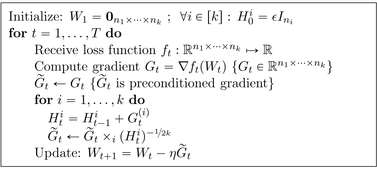
Algorithm 2 maintains one Gram accumulator per mode of an order-k gradient and applies its inverse 1/(2k) power along that mode. Theorem 10 extends the regret bound using the geometric mean of bounds on the ranks of all matricizations. Its trace product has O(√T) growth under the stated boundedness conditions. As in the matrix case, the unprojected algorithm’s comparator-distance term remains an assumption-dependent quantity rather than an automatic constant.

Complete original alg2 from the exact-version PDF, including every panel, label, and original color.
Algorithm 2: Shampoo, general tensor case.
Accessible original algorithm markup

 Initialize: W1=𝟎n1×⋯×nkW_{1}=\bm{0}_{n_{1}\times\cdots\times n_{k}} ;  ∀i∈[k]:H0i=ϵ​Ini\forall i\in[k]:\,H^{i}_{0}=\epsilon I_{n_{i}}  for t=1,…,Tt=1,\ldots,T do   Receive loss function ft:ℝn1×⋯×nk↦ℝf_{t}:\mathbb{R}^{n_{1}\times\cdots\times n_{k}}\mapsto\mathbb{R}   Compute gradient Gt=∇ft​(Wt)G_{t}=\nabla\mkern-1.0muf_{t}(W_{t}) {Gt∈ℝn1×⋯×nkG_{t}\in\mathbb{R}^{n_{1}\times\cdots\times n_{k}}}   G~t←Gt\smash{\widetilde{G}}_{t}\leftarrow G_{t} {G~t\smash{\widetilde{G}}_{t} is preconditioned gradient}   for i=1,…,ki=1,\ldots,k do    Hti=Ht−1i+Gt(i)H^{i}_{t}=H^{i}_{t-1}+G_{t}^{(i)}    G~t←G~t×i(Hti)−1/2​k\smash{\widetilde{G}}_{t}\leftarrow\smash{\widetilde{G}}_{t}\times_{i}(H^{i}_{t})^{-\nicefrac{{1}}{{2k}}}   Update: Wt+1=Wt−η​G~tW_{t+1}=W_{t}-\eta\smash{\widetilde{G}}_{t}

Theorem 10.

Assume that for all i∈[k]i\in[k] and t=1,…,Tt=1,\ldots,T it holds that rank⁡(mati​(Gt))≤ri\mathrm{rank}(\mathrm{mat}_{i}(G_{t}))\leq r_{i}, and let r=(∏i=1kri)1/kr=(\prod_{i=1}^{k}r_{i})^{\nicefrac{{1}}{{k}}}. Then the regret of Algorithm 2 compared to any W⋆∈ℝn1×⋯×nkW^{\star}\in\mathbb{R}^{n_{1}\times\cdots\times n_{k}} is

Equation
∑t=1Tft(Wt)−∑t=1Tft(W⋆)≤2​rD∏i=1kTr((HTi)1/2​k),\displaystyle\sum_{t=1}^{T}f_{t}(W_{t})-\sum_{t=1}^{T}f_{t}(W^{\star})\leq\sqrt{2r}D\prod_{i=1}^{k}\trace\mathopen{}\big((H_{T}^{i})^{\nicefrac{{1}}{{2k}}}\big),

where HTi=ϵ​Ini+∑t=1TGt(i)H_{T}^{i}=\epsilon I_{n_{i}}+\sum_{t=1}^{T}G_{t}^{(i)} for all i∈[k]i\in[k] and D=maxt∈[T]⁡‖Wt−W⋆‖𝖥D=\max_{t\in[T]}\|W_{t}-W^{\star}\|_{\mathsf{F}}.

4.3 Analysis

Lemma 11 compares the accumulated outer products of flattened gradients with a Kronecker product of mode-wise accumulators, including the geometric-mean rank factor. Lemma 12 proves that applying a Kronecker product to a flattened tensor equals applying the corresponding matrices along its modes. Together they convert Algorithm 2 to mirror descent with an implicit metric, so the matrix proof extends. Appendix B supplies the technical details rather than leaving this tensor generalization merely intuitive.

Lemma 11.

Assume that G1,…,GTG_{1},\ldots,G_{T} are all order kk tensors of dimension n1×⋯×nkn_{1}\times\cdots\times n_{k}, and let n=n1⋯nkn=n_{1}\cdots n_{k} and gt=vec¯​(Gt)g_{t}=\overline{\mathrm{vec}}(G_{t}) for all tt. Let rir_{i} denote the bound on the rank of the ithi^{\footnotesize\mbox{th}} matricization of G1,…,GTG_{1},\ldots,G_{T}, namely, rank⁡(mati​(Gt))≤ri\mathrm{rank}(\mathrm{mat}_{i}(G_{t}))\leq r_{i} for all tt and i∈[k]i\in[k]. Denote r=(∏i=1kri)1/kr=(\prod_{i=1}^{k}r_{i})^{\nicefrac{{1}}{{k}}}. Then, for any ϵ≥0\epsilon\geq 0 it holds that

Equation
ϵIn+∑t=1Tgtgt𝖳⪯r⨂i=1k(ϵIni+∑t=1TGt(i))1/k.\displaystyle\epsilon I_{n}+\sum_{t=1}^{T}g_{t}g_{t}^{\mkern-1.5mu\scriptstyle\mathsf{T}}~\preceq~r\,\bigotimes_{i=1}^{k}\mathopen{}\Big(\epsilon I_{n_{i}}+\sum_{t=1}^{T}G_{t}^{(i)}\Big)^{\nicefrac{{1}}{{k}}}~.
Lemma 12.

Let GG be an n1×…×nkn_{1}\times\ldots\times n_{k} dimensional tensor and MiM_{i} be an ni×nin_{i}\times n_{i} for i∈[k]i\in[k] , then

Equation
(⨂i=1kMi)vec¯(G)=vec¯(G×1M1×2M2…×kMk).\displaystyle\mathopen{}\Big(\bigotimes_{i=1}^{k}M_{i}\Big)\overline{\mathrm{vec}}(G)=\overline{\mathrm{vec}}(G\times_{1}M_{1}\times_{2}M_{2}\ldots\times_{k}M_{k})~.
Equation
Ht=(⨂i=1kHti)1/2​k,gt=vec¯​(Gt),wt=vec¯​(Wt).H_{t}=(\bigotimes_{i=1}^{k}H_{t}^{i})^{\nicefrac{{1}}{{2k}}}~~,~~g_{t}=\overline{\mathrm{vec}}(G_{t})~~,~~w_{t}=\overline{\mathrm{vec}}(W_{t})~.

5 Implementation details

The TensorFlow implementation uses tensor contractions and SVD-based matrix powers. It treats each model tensor separately, so the overall preconditioner is block diagonal across tensors: cross-tensor correlations are ignored. For an excessively large mode, it switches only that mode to diagonal preconditioning, using a threshold near 1,200 in these experiments. This limits memory and factorization costs without requiring every other mode to become diagonal.

6 Experimental results

The practical experiments use batch size 128, momentum 0.9, and roots recomputed every 20–100 steps. Accumulators are updated from averaged mini-batch gradients, not separate outer products for every example. These choices change the exact theoretical pseudocode and are evaluated empirically. Table 1 reports throughput on a Tesla K40. Shampoo has similar throughput on the image models, but the language-model case is 3.509 steps/s versus Adam’s4.871; faster progress per step should not be presented as automatically faster wall-clock convergence.

Dataset SGD Adam AdaGrad Shampoo
CIFAR10 (ResNet-32) 2.184 2.184 2.197 2.151
CIFAR10 (Inception) 3.638 3.667 3.682 3.506
CIFAR100 (ResNet-55) 1.210 1.203 1.210 1.249
LM1B (Attention) 4.919 4.871 4.908 3.509
Table 1: Average number of steps per second (with batch size of 128) in each experiment, for each of the algorithms we tested.

6.1 Image Classification

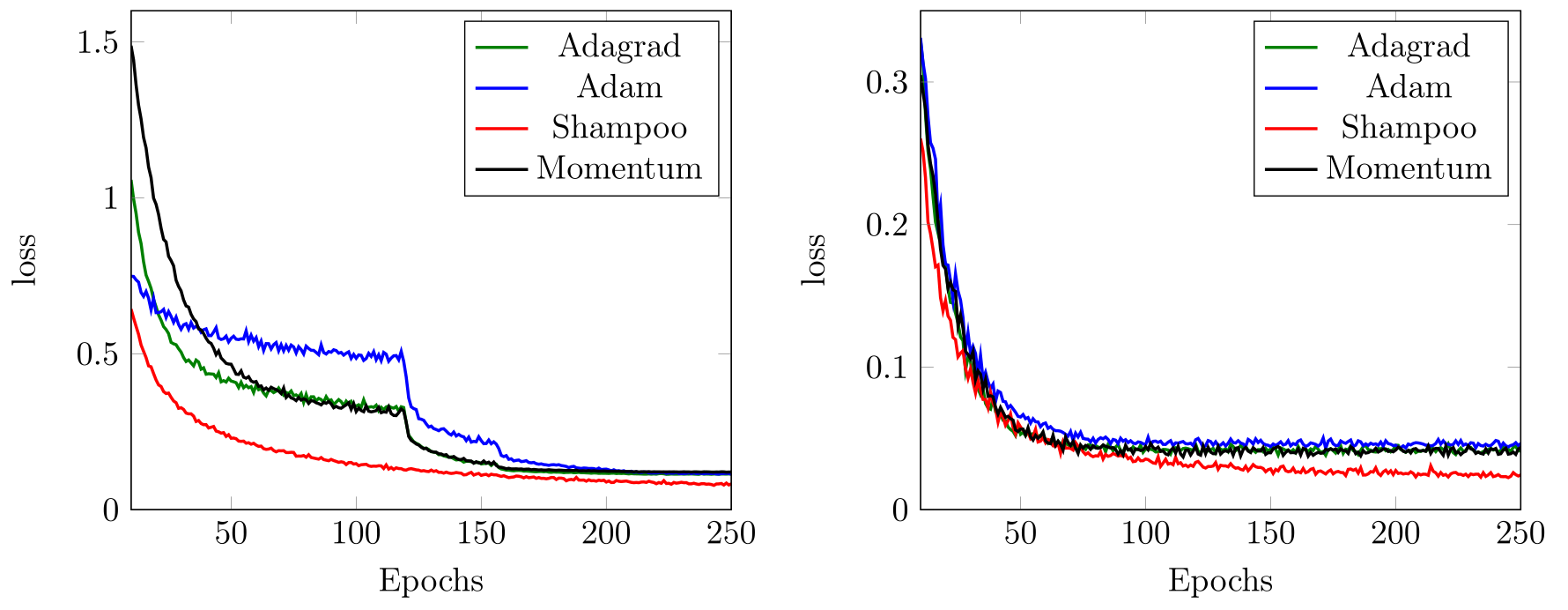
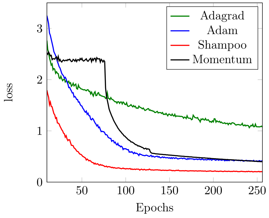
The image experiments compare learning curves for residual and inception networks on CIFAR-10 and a residual network without batch normalization on CIFAR-100. Each optimizer receives a learning-rate sweep, and the figures show training loss against epochs. The text gives test-error levels reached by these architectures, but the plots are not replicated test-accuracy comparisons with uncertainty intervals. They support the reported optimization behavior in these settings rather than universal superiority across architectures.

Complete original S6.F2 from the exact-version PDF, including every panel, label, and original color.
Figure 2: Training loss for a residual network and an inception network on CIFAR-10.
Complete original S6.F3 from the exact-version PDF, including every panel, label, and original color.
Figure 3: Training loss for a residual network on CIFAR-100 (without batchnorm).

6.2 Language Models

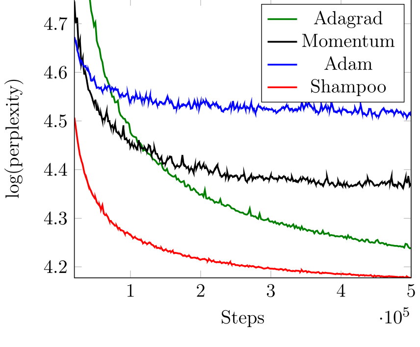
The LM1B experiment uses a 9.8M-parameter attention model and plots test log-perplexity against steps. Shampoo uses its default learning rate 1.0 while alternatives receive several learning-rate settings. The observed curve improves faster in steps, but the throughput table shows a meaningful per-step cost. This historical small-model experiment does not establish compute savings for today’s large language-model pretraining.

Complete original S6.F4 from the exact-version PDF, including every panel, label, and original color.
Figure 4: Test log-perplexity of an Attention model of Vaswani et al. [22].

Acknowledgements

The acknowledgements credit colleagues for technical discussions and the optimizer’s name.

Appendix A Diagonal Shampoo

Diagonal Shampoo keeps only each mode accumulator’s diagonal. In the matrix case this uses O(m+n) preconditioner storage and O(mn) update time; it can also be mixed with full preconditioning on another mode. Theorem 13 replaces the Frobenius comparator-distance factor with an entrywise infinity-norm factor. Its proof adapts the changing-metric term using diagonal PSD matrices and applies diagonal extraction to the structured/full-moment comparison. The complete Algorithm 3 and formal bound are retained.

Equation
Lt\displaystyle L_{t} =Lt−1+diag(Gt​Gt𝖳);\displaystyle=L_{t-1}+\diag(G_{t}G_{t}^{\mkern-1.5mu\scriptstyle\mathsf{T}});
Rt\displaystyle R_{t} =Rt−1+diag(Gt𝖳​Gt).\displaystyle=R_{t-1}+\diag(G_{t}^{\mkern-1.5mu\scriptstyle\mathsf{T}}G_{t}).
Complete original alg3 from the exact-version PDF, including every panel, label, and original color.
Algorithm 3: Diagonal version of Shampoo, matrix case.
Accessible original algorithm markup

 Initialize W1=𝟎m×n;L0=ϵ​Im;R0=ϵ​InW_{1}=\bm{0}_{m\times n}~;~L_{0}=\epsilon I_{m}~;~R_{0}=\epsilon I_{n}  for t=1,…,Tt=1,\ldots,T do   Receive loss function ft:ℝm×n↦ℝf_{t}:\mathbb{R}^{m\times n}\mapsto\mathbb{R}   Compute gradient Gt=∇ft​(Wt)G_{t}=\nabla\mkern-1.0muf_{t}(W_{t}) {Gt∈ℝm×nG_{t}\in\mathbb{R}^{m\times n}}   Update preconditioners:

Equation Lt\displaystyle L_{t} =Lt−1+diag(Gt​Gt𝖳)\displaystyle=L_{t-1}+\diag(G_{t}G_{t}^{\mkern-1.5mu\scriptstyle\mathsf{T}}) Rt\displaystyle R_{t} =Rt−1+diag(Gt𝖳​Gt)\displaystyle=R_{t-1}+\diag(G_{t}^{\mkern-1.5mu\scriptstyle\mathsf{T}}G_{t})
  Update parameters:
EquationWt+1=Wt−η​Lt−1/4​Gt​Rt−1/4W_{t+1}~=~W_{t}-\eta L_{t}^{-\nicefrac{{1}}{{4}}}G_{t}R_{t}^{-\nicefrac{{1}}{{4}}}

Theorem 13.

Assume that the gradients G1,…,GTG_{1},\ldots,G_{T} are matrices of rank at most rr. Then the regret of Algorithm 3 compared to any W⋆∈ℝm×nW^{\star}\in\mathbb{R}^{m\times n} is bounded as

Equation
∑t=1Tft(Wt)−∑t=1Tft(W⋆)≤2​rD∞Tr(LT1/4)Tr(RT1/4),\displaystyle\sum_{t=1}^{T}f_{t}(W_{t})-\sum_{t=1}^{T}f_{t}(W^{\star})\leq\sqrt{2r}D_{\infty}\trace(L_{T}^{{\smash{\nicefrac{{1}}{{4}}}}})\trace(R_{T}^{{\smash{\nicefrac{{1}}{{4}}}}})~,

where

Equation
LT=ϵ​Im+∑t=1Tdiag(Gt​Gt𝖳),RT=ϵ​In+∑t=0Tdiag(Gt𝖳​Gt),D∞=maxt∈[T]⁡‖Wt−W⋆‖∞.L_{T}=\epsilon I_{m}+\sum_{t=1}^{T}\diag(G_{t}G_{t}^{\mkern-1.5mu\scriptstyle\mathsf{T}})\;,\;\;R_{T}=\epsilon I_{n}+\sum_{t=0}^{T}\diag(G_{t}^{\mkern-1.5mu\scriptstyle\mathsf{T}}G_{t})\;,\;\;D_{\infty}=\max_{t\in[T]}\|W_{t}-W^{\star}\|_{\infty}~.

(Here, ‖A‖∞\|A\|_{\infty} is the entry-wise ℓ∞\ell_{\infty} norm of a matrix AA, i.e., ‖A‖∞=def‖vec¯​(A)‖∞\|A\|_{\infty}\stackrel{{\scriptstyle\text{def}}}{{=}}\|\overline{\mathrm{vec}}(A)\|_{\infty}.)

Equations
∑t=1T(wt−w⋆)𝖳(Ht−Ht−1)(wt−w⋆)≤D∞2∑t=1TTr(Ht−Ht−1)=D∞2Tr(HT),\displaystyle\sum_{t=1}^{T}(w_{t}-w^{\star})^{\mkern-1.5mu\scriptstyle\mathsf{T}}(H_{t}-H_{t-1})(w_{t}-w^{\star})\leq D_{\infty}^{2}\sum_{t=1}^{T}\trace(H_{t}-H_{t-1})=D_{\infty}^{2}\trace(H_{T})~,
H^t=defdiag(rϵIm​n+∑s=1tgtgt𝖳)1/2⪯rLt1/4⊗Rt1/4=rHt,\displaystyle\smash{\widehat{H}}_{t}\stackrel{{\scriptstyle\text{def}}}{{=}}\diag\mathopen{}\Big(r\epsilon I_{mn}+\sum_{s=1}^{t}g_{t}g_{t}^{\mkern-1.5mu\scriptstyle\mathsf{T}}\Big)^{{\smash{\nicefrac{{1}}{{2}}}}}\preceq\sqrt{r}L_{t}^{{\smash{\nicefrac{{1}}{{4}}}}}\otimes R_{t}^{{\smash{\nicefrac{{1}}{{4}}}}}=\sqrt{r}H_{t}~,

Appendix B Tensor case: Technical proofs

Lemma 14 establishes the tensor identities needed by the later proofs. It verifies vectorization and matricization on rank-one outer products, proves the boundary-mode vectorization equalities, and checks how mode multiplication appears after matricization. Linearity then extends these identities to arbitrary tensors. These bookkeeping steps preserve the ordering convention that the Kronecker proof requires.

Lemma 14.

For any column vectors u1,…,uku^{1},\ldots,u^{k} and order-kk tensor AA it holds that:

  1. (i)

    vec¯(u1∘⋯∘uk)=u1⊗⋯⊗uk\overline{\mathrm{vec}}(u^{1}\circ\cdots\circ u^{k})=u^{1}\otimes\cdots\otimes u^{k}  ;

  2. (ii)

    mati(u1∘⋯∘uk)=ui(⨂i′≠iui′)𝖳\mathrm{mat}_{i}(u^{1}\circ\cdots\circ u^{k})=u^{i}\big(\bigotimes_{i^{\prime}\neq i}u^{i^{\prime}}\big)^{\mkern-1.5mu\scriptstyle\mathsf{T}}   ;

  3. (iii)

    vec¯​(A)=vec¯​(mat1​(A))=vec¯​(matk​(A)𝖳)\overline{\mathrm{vec}}(A)=\overline{\mathrm{vec}}(\mathrm{mat}_{1}(A))=\overline{\mathrm{vec}}(\mathrm{mat}_{k}(A)^{\mkern-1.5mu\scriptstyle\mathsf{T}})   ;

  4. (iv)

    mati​(A×iM)=M​mati​(A)\mathrm{mat}_{i}(A\times_{i}M)=M\mathrm{mat}_{i}(A)  .

Equations
vec¯(u1∘⋯∘uk)\displaystyle\overline{\mathrm{vec}}(u^{1}\circ\cdots\circ u^{k})
=(u11(u2⊗⋯⊗uk)𝖳,⋯,un11(u2⊗⋯⊗uk)𝖳)𝖳\displaystyle=(u^{1}_{1}(u^{2}\otimes\cdots\otimes u^{k})^{\mkern-1.5mu\scriptstyle\mathsf{T}},\cdots,u^{1}_{n_{1}}(u^{2}\otimes\cdots\otimes u^{k})^{\mkern-1.5mu\scriptstyle\mathsf{T}})^{\mkern-1.5mu\scriptstyle\mathsf{T}}
=u1⊗⋯⊗uk.\displaystyle=u^{1}\otimes\cdots\otimes u^{k}.
mati(u1∘⋯∘uk)=(u1i⨂j≠iuj,…,unii⨂j≠iuj)𝖳=ui(⨂j≠iuj)𝖳.\displaystyle\mathrm{mat}_{i}(u^{1}\circ\cdots\circ u^{k})=\mathopen{}\Big(u^{i}_{1}\bigotimes_{j\neq i}u^{j},\ldots,u^{i}_{n_{i}}\bigotimes_{j\neq i}u^{j}\Big)^{\mkern-1.5mu\scriptstyle\mathsf{T}}=u^{i}\mathopen{}\Big(\bigotimes_{j\neq i}u^{j}\Big)^{\mkern-1.5mu\scriptstyle\mathsf{T}}.
vec¯​(mat1​(A))\displaystyle\overline{\mathrm{vec}}(\mathrm{mat}_{1}(A)) =vec¯(u1(u2⊗⋯⊗uk)𝖳)\displaystyle=\overline{\mathrm{vec}}(u^{1}(u^{2}\otimes\cdots\otimes u^{k})^{\mkern-1.5mu\scriptstyle\mathsf{T}})
=u1⊗⋯⊗uk=vec¯(A),\displaystyle=u^{1}\otimes\cdots\otimes u^{k}=\overline{\mathrm{vec}}(A)~,
vec¯​(matk​(A)𝖳)\displaystyle\overline{\mathrm{vec}}(\mathrm{mat}_{k}(A)^{\mkern-1.5mu\scriptstyle\mathsf{T}}) =vec¯((uk(u1⊗⋯⊗uk−1)𝖳)𝖳)\displaystyle=\overline{\mathrm{vec}}((u^{k}(u^{1}\otimes\cdots\otimes u^{k-1})^{\mkern-1.5mu\scriptstyle\mathsf{T}})^{\mkern-1.5mu\scriptstyle\mathsf{T}})
=vec¯((u1⊗⋯⊗uk−1)(uk)𝖳)\displaystyle=\overline{\mathrm{vec}}((u^{1}\otimes\cdots\otimes u^{k-1})(u^{k})^{\mkern-1.5mu\scriptstyle\mathsf{T}})
=u1⊗⋯⊗uk=vec¯(A).\displaystyle=u^{1}\otimes\cdots\otimes u^{k}=\overline{\mathrm{vec}}(A)~.
A×iM=u1∘⋯∘ui−1∘Mui∘ui+1∘⋯∘uk.\displaystyle A\times_{i}M=u^{1}\circ\cdots\circ u^{i-1}\circ Mu^{i}\circ u^{i+1}\circ\cdots\circ u^{k}~.
mati(A×iM)=Mui(⨂j≠iuj)𝖳=Mmati(A).\displaystyle\mathrm{mat}_{i}(A\times_{i}M)=Mu^{i}\mathopen{}\Big(\bigotimes_{j\neq i}u^{j}\Big)^{\mkern-1.5mu\scriptstyle\mathsf{T}}=M\mathrm{mat}_{i}(A)~.

B.1 Proof of Lemma 11

Lemma 15 shows that a PSD inequality expressed after one matricization is equivalent to the corresponding inequality in the canonical tensor flattening. The proof evaluates both quadratic forms on an arbitrary test tensor and expands coordinates to show equality. Applying the matrix rank bound to each matricized gradient, transporting it back, and summing over time yields one inequality per mode. Their right-hand factors commute, so the geometric-mean inequality combines them into Lemma 11 with its rank multiplier.

Lemma 15.

Let GG be an order kk tensor of dimension n1×⋯×nkn_{1}\times\cdots\times n_{k}, and BB an ni×nin_{i}\times n_{i} matrix. Let gi=vec¯​(mati​(G))g_{i}=\overline{\mathrm{vec}}(\mathrm{mat}_{i}(G)) and g=vec¯​(G)g=\overline{\mathrm{vec}}(G). Then

Equation
gigi𝖳⪯B⊗(⨂j≠iInj)⇔gg𝖳⪯(⨂j<iInj)⊗B⊗(⨂j>iInj).\displaystyle g_{i}g_{i}^{\mkern-1.5mu\scriptstyle\mathsf{T}}\preceq B\otimes\mathopen{}\Big(\bigotimes_{j\neq i}I_{n_{j}}\Big)~~~\Leftrightarrow~~~gg^{\mkern-1.5mu\scriptstyle\mathsf{T}}\preceq\mathopen{}\Big(\bigotimes_{j<i}I_{n_{j}}\Big)\otimes B\otimes\mathopen{}\Big(\bigotimes_{j>i}I_{n_{j}}\Big).
Equations
x=vec¯​(X),xi=vec¯​(mati​(X)).x=\overline{\mathrm{vec}}(X)~,~x_{i}=\overline{\mathrm{vec}}(\mathrm{mat}_{i}(X))~.
xi𝖳gigi𝖳xi≤xi𝖳[B⊗(⨂j≠iInj)]xi⇔x𝖳gg𝖳x≤x𝖳[(⨂j<iInj)⊗B⊗(⨂j>iInj)]x,\displaystyle x_{i}^{\mkern-1.5mu\scriptstyle\mathsf{T}}g_{i}g_{i}^{\mkern-1.5mu\scriptstyle\mathsf{T}}x_{i}\leq x_{i}^{\mkern-1.5mu\scriptstyle\mathsf{T}}\mathopen{}\Big[B\otimes\mathopen{}\Big(\bigotimes_{j\neq i}I_{n_{j}}\Big)\Big]x_{i}~~~\Leftrightarrow~~~x^{\mkern-1.5mu\scriptstyle\mathsf{T}}gg^{\mkern-1.5mu\scriptstyle\mathsf{T}}x\leq x^{\mkern-1.5mu\scriptstyle\mathsf{T}}\mathopen{}\Big[\mathopen{}\Big(\bigotimes_{j<i}I_{n_{j}}\Big)\otimes B\otimes\mathopen{}\Big(\bigotimes_{j>i}I_{n_{j}}\Big)\Big]x~,
x𝖳[(⨂j<iInj)⊗B⊗(⨂j>iInj)]x\displaystyle x^{\mkern-1.5mu\scriptstyle\mathsf{T}}\mathopen{}\Big[\mathopen{}\Big(\bigotimes_{j<i}I_{n_{j}}\Big)\otimes B\otimes\mathopen{}\Big(\bigotimes_{j>i}I_{n_{j}}\Big)\Big]x =x𝖳∑αXα[(⨂j<iInj)⊗B⊗(⨂j>iInj)](eα1⊗⋯⊗eαk)\displaystyle=x^{\mkern-1.5mu\scriptstyle\mathsf{T}}\sum_{\alpha}X_{\alpha}\mathopen{}\Big[\mathopen{}\Big(\bigotimes_{j<i}I_{n_{j}}\Big)\otimes B\otimes\mathopen{}\Big(\bigotimes_{j>i}I_{n_{j}}\Big)\Big](e_{\alpha_{1}}\otimes\cdots\otimes e_{\alpha_{k}})
=x𝖳∑αXα[(⨂j<ieαj)⊗Beαi⊗(⨂j>ieαj)]\displaystyle=x^{\mkern-1.5mu\scriptstyle\mathsf{T}}\sum_{\alpha}X_{\alpha}\mathopen{}\Big[\mathopen{}\Big(\bigotimes_{j<i}e_{\alpha_{j}}\Big)\otimes Be_{\alpha_{i}}\otimes\mathopen{}\Big(\bigotimes_{j>i}e_{\alpha_{j}}\Big)\Big]
=∑α,α′XαXα′[(⨂j<ieαj′𝖳eαj)⊗eαi′𝖳Beαi⊗(⨂j>ieαj′𝖳eαj)]\displaystyle=\sum_{\alpha,\alpha^{\prime}}X_{\alpha}X_{\alpha^{\prime}}\mathopen{}\Big[\mathopen{}\Big(\bigotimes_{j<i}e_{\smash{\alpha^{\prime}_{j}}}^{\mkern-1.5mu\scriptstyle\mathsf{T}}e_{\smash{\alpha_{j}}}\Big)\otimes e_{\smash{\alpha^{\prime}_{i}}}^{\mkern-1.5mu\scriptstyle\mathsf{T}}Be_{\alpha_{i}}\otimes\mathopen{}\Big(\bigotimes_{j>i}e_{\smash{\alpha^{\prime}_{j}}}^{\mkern-1.5mu\scriptstyle\mathsf{T}}e_{\alpha_{j}}\Big)\Big]
=∑α,αi′Bαi′​αi​Xα1​…​αi​…​αk​Xα1​…​αi′​…​αk,\displaystyle=\sum_{\alpha,\alpha^{\prime}_{i}}B_{\alpha^{\prime}_{i}\alpha_{i}}X_{\alpha_{1}\ldots\alpha_{i}\ldots\alpha_{k}}X_{\alpha_{1}\ldots\alpha^{\prime}_{i}\ldots\alpha_{k}},
mati(X)=∑αXαeαi(⨂j≠ieαj)𝖳,\mathrm{mat}_{i}(X)=\sum_{\alpha}X_{\alpha}e_{\alpha_{i}}\mathopen{}\Big(\bigotimes_{j\neq i}e_{\alpha_{j}}\Big)^{\mkern-1.5mu\scriptstyle\mathsf{T}},
xi=vec¯(mati(X))=∑αXα(eαi⊗⨂j≠ieαj)x_{i}=\overline{\mathrm{vec}}(\mathrm{mat}_{i}(X))=\sum_{\alpha}X_{\alpha}\mathopen{}\Big(e_{\alpha_{i}}\otimes\bigotimes_{j\neq i}e_{\alpha_{j}}\Big)
xi𝖳[B⊗(⨂j≠iInj)]xi\displaystyle x_{i}^{\mkern-1.5mu\scriptstyle\mathsf{T}}\mathopen{}\Big[B\otimes\mathopen{}\Big(\bigotimes_{j\neq i}I_{n_{j}}\Big)\Big]x_{i} =xi𝖳∑αXα[B⊗(⨂j≠iInj)](eαi⊗⨂j≠ieαj)\displaystyle=x_{i}^{\mkern-1.5mu\scriptstyle\mathsf{T}}\sum_{\alpha}X_{\alpha}\mathopen{}\Big[B\otimes\mathopen{}\Big(\bigotimes_{j\neq i}I_{n_{j}}\Big)\Big]\mathopen{}\Big(e_{\alpha_{i}}\otimes\bigotimes_{j\neq i}e_{\alpha_{j}}\Big)
=xi𝖳∑αXα(Beαi⊗⨂j≠ieαj)\displaystyle=x_{i}^{\mkern-1.5mu\scriptstyle\mathsf{T}}\sum_{\alpha}X_{\alpha}\mathopen{}\Big(Be_{\alpha_{i}}\otimes\bigotimes_{j\neq i}e_{\alpha_{j}}\Big)
=∑α′∑αXαXα′(eαi′𝖳Beαi⊗⨂j≠ieαj′𝖳eαj)\displaystyle=\sum_{\alpha^{\prime}}\sum_{\alpha}X_{\alpha}X_{\alpha^{\prime}}\mathopen{}\Big(e_{\smash{\alpha^{\prime}_{i}}}^{\mkern-1.5mu\scriptstyle\mathsf{T}}Be_{\alpha_{i}}\otimes\bigotimes_{j\neq i}e_{\smash{\alpha^{\prime}_{j}}}^{\mkern-1.5mu\scriptstyle\mathsf{T}}e_{\alpha_{j}}\Big)
=∑α,αi′Bαi′​αi​Xα1​…​αi​…​αk​Xα1​…​αi′​…​αk.\displaystyle=\sum_{\alpha,\alpha^{\prime}_{i}}B_{\alpha^{\prime}_{i}\alpha_{i}}X_{\alpha_{1}\ldots\alpha_{i}\ldots\alpha_{k}}X_{\alpha_{1}\ldots\alpha^{\prime}_{i}\ldots\alpha_{k}}.
xi𝖳[B⊗(⨂j≠iInj)]xi=x𝖳[(⨂j<iInj)⊗B⊗(⨂j>iInj)]x,\displaystyle x_{i}^{\mkern-1.5mu\scriptstyle\mathsf{T}}\mathopen{}\Big[B\otimes\mathopen{}\Big(\bigotimes_{j\neq i}I_{n_{j}}\Big)\Big]x_{i}=x^{\mkern-1.5mu\scriptstyle\mathsf{T}}\mathopen{}\Big[\mathopen{}\Big(\bigotimes_{j<i}I_{n_{j}}\Big)\otimes B\otimes\mathopen{}\Big(\bigotimes_{j>i}I_{n_{j}}\Big)\Big]x,
1rivec¯(mati(Gt))vec¯(mati(Gt))𝖳⪯(mati(Gt)mati(Gt)𝖳)⊗In−i=Gt(i)⊗(⨂j≠iInj)\displaystyle\frac{1}{r_{i}}\overline{\mathrm{vec}}(\mathrm{mat}_{i}(G_{t}))\overline{\mathrm{vec}}(\mathrm{mat}_{i}(G_{t}))^{\mkern-1.5mu\scriptstyle\mathsf{T}}\preceq(\mathrm{mat}_{i}(G_{t})\mathrm{mat}_{i}(G_{t})^{\mkern-1.5mu\scriptstyle\mathsf{T}})\otimes I_{n_{-i}}=G_{t}^{(i)}\otimes\mathopen{}\Big(\bigotimes_{j\neq i}I_{n_{j}}\Big)
1rigtgt𝖳⪯(⨂j=1i−1Inj)⊗Gt(i)⊗(⨂j=i+1kInj).\displaystyle\frac{1}{r_{i}}g_{t}g_{t}^{\mkern-1.5mu\scriptstyle\mathsf{T}}\preceq\mathopen{}\Big(\bigotimes_{j=1}^{i-1}I_{n_{j}}\Big)\otimes G_{t}^{(i)}\otimes\mathopen{}\Big(\bigotimes_{j=i+1}^{k}I_{n_{j}}\Big).
ϵ​In+∑t=1Tgt​gt𝖳\displaystyle\epsilon I_{n}+\sum_{t=1}^{T}g_{t}g_{t}^{\mkern-1.5mu\scriptstyle\mathsf{T}} ⪯riϵIn+ri(⨂j=1i−1Inj)⊗(∑t=1TGt(i))⊗(⨂j=i+1kInj)\displaystyle\preceq r_{i}\epsilon I_{n}+r_{i}\,\mathopen{}\Big(\bigotimes_{j=1}^{i-1}I_{n_{j}}\Big)\otimes\mathopen{}\Big(\sum_{t=1}^{T}G_{t}^{(i)}\Big)\otimes\mathopen{}\Big(\bigotimes_{j=i+1}^{k}I_{n_{j}}\Big)
=ri(⨂j=1i−1Inj)⊗(ϵIni+∑t=1TGt(i))⊗(⨂j=i+1kInj).\displaystyle=r_{i}\,\mathopen{}\Big(\bigotimes_{j=1}^{i-1}I_{n_{j}}\Big)\otimes\mathopen{}\Big(\epsilon I_{n_{i}}+\sum_{t=1}^{T}G_{t}^{(i)}\Big)\otimes\mathopen{}\Big(\bigotimes_{j=i+1}^{k}I_{n_{j}}\Big).

B.2 Proof of Lemma 12

The proof of Lemma 12 inducts on tensor order. It isolates the last mode through its matricization, applies the matrix vectorization identity, and uses the induction hypothesis independently on each lower-order slice. Stacking those slices and restoring the last mode gives the full Kronecker/mode-multiplication identity. The original displayed chain retains the transposes that make the dimensions consistent.

Equations
(⨂i=1kMi)vec¯(G)=(H⊗Mk)vec¯(matk(G)𝖳)=vec¯(Hmatk(G)𝖳Mk𝖳).\displaystyle\mathopen{}\Big(\bigotimes_{i=1}^{k}M_{i}\Big)\overline{\mathrm{vec}}(G)=(H\otimes M_{k})\overline{\mathrm{vec}}(\mathrm{mat}_{k}(G)^{\mkern-1.5mu\scriptstyle\mathsf{T}})=\overline{\mathrm{vec}}(H\mathrm{mat}_{k}(G)^{\mkern-1.5mu\scriptstyle\mathsf{T}}M_{k}^{\mkern-1.5mu\scriptstyle\mathsf{T}}).
Hvec¯(Gik)=(⨂i=1k−1Mi)vec¯(Gik)=vec¯(Gik×1M1×2M2⋯×k−1Mk−1).\displaystyle H\overline{\mathrm{vec}}(G^{k}_{i})=\mathopen{}\Big(\bigotimes_{i=1}^{k-1}M_{i}\Big)\overline{\mathrm{vec}}(G^{k}_{i})=\overline{\mathrm{vec}}(G^{k}_{i}\times_{1}M_{1}\times_{2}M_{2}\cdots\times_{k-1}M_{k-1}).
Hmatk(G)𝖳=matk(G×1M1×2M2⋯×k−1Mk−1)𝖳.H\mathrm{mat}_{k}(G)^{\mkern-1.5mu\scriptstyle\mathsf{T}}=\mathrm{mat}_{k}(G\times_{1}M_{1}\times_{2}M_{2}\cdots\times_{k-1}M_{k-1})^{\mkern-1.5mu\scriptstyle\mathsf{T}}.
(⨂i=1kMi)vec¯(G)\displaystyle\smash{\mathopen{}\Big(\bigotimes_{i=1}^{k}M_{i}\Big)}\overline{\mathrm{vec}}(G) =vec¯​(matk​(G′)𝖳​Mk𝖳)\displaystyle=\overline{\mathrm{vec}}(\mathrm{mat}_{k}(G^{\prime})^{\mkern-1.5mu\scriptstyle\mathsf{T}}M_{k}^{\mkern-1.5mu\scriptstyle\mathsf{T}})
=vec¯​((Mk​matk​(G′))𝖳)\displaystyle=\overline{\mathrm{vec}}((M_{k}\mathrm{mat}_{k}(G^{\prime}))^{\mkern-1.5mu\scriptstyle\mathsf{T}})
=vec¯​(matk​(G′×kMk)𝖳)\displaystyle=\overline{\mathrm{vec}}(\mathrm{mat}_{k}(G^{\prime}\times_{k}M_{k})^{\mkern-1.5mu\scriptstyle\mathsf{T}}) ∵B​mati​(A)=mati​(A×iB)\displaystyle\qquad\because~B\mathrm{mat}_{i}(A)=\mathrm{mat}_{i}(A\times_{i}B)
=vec¯​(G′×kMk)\displaystyle=\overline{\mathrm{vec}}(G^{\prime}\times_{k}M_{k}) ∵vec¯​(matk​(G)𝖳)=vec¯​(G)\displaystyle\qquad\because~\overline{\mathrm{vec}}(\mathrm{mat}_{k}(G)^{\mkern-1.5mu\scriptstyle\mathsf{T}})=\overline{\mathrm{vec}}(G)
=vec¯(G×1M1⋯×kMk).\displaystyle=\overline{\mathrm{vec}}(G\times_{1}M_{1}\cdots\times_{k}M_{k}).

Appendix C Additional proofs

C.1 Proof of Lemma 2

Lemma 2 follows a follow-the-leader/be-the-leader induction. The potential-minimizing metric at the preceding round cannot improve the previous objective over its minimizer; substituting the final-round metric and adding the new dual-gradient term yields the desired telescoping comparison. The existence of each metric minimizer is an explicit assumption in the lemma.

Equations
∑t=1T(∥gt∥Ht∗)2+Φ(H0)≤∑t=1T(∥gt∥HT∗)2+Φ(HT).\displaystyle\sum_{t=1}^{T}\mathopen{}\big(\|g_{t}\|_{H_{t}}^{*}\big)^{2}+\Phi(H_{0})~\leq~\sum_{t=1}^{T}\mathopen{}\big(\|g_{t}\|_{H_{T}}^{*}\big)^{2}+\Phi(H_{T})~.
∑t=1T−1(∥gt∥Ht∗)2+Φ(H0)\displaystyle\sum_{t=1}^{T-1}\mathopen{}\big(\|g_{t}\|_{H_{t}}^{*}\big)^{2}+\Phi(H_{0}) ≤∑t=1T−1(∥gt∥HT−1∗)2+Φ(HT−1)\displaystyle~\leq~\sum_{t=1}^{T-1}\mathopen{}\big(\|g_{t}\|_{H_{T-1}}^{*}\big)^{2}+\Phi(H_{T-1})
≤∑t=1T−1(∥gt∥HT∗)2+Φ(HT).\displaystyle~\leq~\sum_{t=1}^{T-1}\mathopen{}\big(\|g_{t}\|_{H_{T}}^{*}\big)^{2}+\Phi(H_{T})~.
MT−1∙H−1+Φ(H)=∑t=1T−1(∥gt∥H∗)2+Φ(H).M_{T-1}\bullet H^{-1}+\Phi(H)=\sum_{t=1}^{T-1}\mathopen{}\big(\|g_{t}\|_{H}^{*}\big)^{2}+\Phi(H)~.

C.2 Proof of Lemma 4

The matrix vectorization identity is proved first for a rank-one matrix. Both the Kronecker expression and the left/right matrix product reduce to the same tensor product of two vectors. Decomposing any matrix into rank-one terms and using linearity completes the proof. This closes the algebraic link underlying the efficient implementation.

Equations
(L⊗R𝖳)​vec¯​(G)\displaystyle(L\otimes R^{\mkern-1.5mu\scriptstyle\mathsf{T}})\overline{\mathrm{vec}}(G) =(L⊗R𝖳)​vec¯​(u​v𝖳)=(L⊗R𝖳)​(u⊗v)=(L​u)⊗(R𝖳​v).\displaystyle=(L\otimes R^{\mkern-1.5mu\scriptstyle\mathsf{T}})\overline{\mathrm{vec}}(uv^{\mkern-1.5mu\scriptstyle\mathsf{T}})=(L\otimes R^{\mkern-1.5mu\scriptstyle\mathsf{T}})(u\otimes v)=(Lu)\otimes(R^{\mkern-1.5mu\scriptstyle\mathsf{T}}v)~.
vec¯​(L​G​R)\displaystyle\overline{\mathrm{vec}}(LGR) =vec¯(Luv𝖳R)=vec¯(Lu(R𝖳v)𝖳)=(Lu)⊗(R𝖳v),\displaystyle=\overline{\mathrm{vec}}(Luv^{\mkern-1.5mu\scriptstyle\mathsf{T}}R)=\overline{\mathrm{vec}}\mathopen{}\big(Lu(R^{\mkern-1.5mu\scriptstyle\mathsf{T}}v)^{\mkern-1.5mu\scriptstyle\mathsf{T}}\big)=(Lu)\otimes(R^{\mkern-1.5mu\scriptstyle\mathsf{T}}v)~,
Concept demonstration

Open image ↗