Overview
At a glance
Intuition. Training has two jobs here: improve predictions and gently shrink weights. Adam rescales each coordinate’s gradient using its recent history. If shrinkage is included inside that gradient, it gets rescaled too, so two equally large weights can receive different shrinkage. AdamW applies shrinkage separately.
Reading the math. As a simple illustration, multiplying weights 2 and 0.2 by 0.99 gives 1.98 and 0.198: the same percentage reduction. Adam’s separate prediction-improving step still uses m, a moving average of gradients, and v, a moving average of squared gradients. These gradient statistics are not the full Fisher metric.
Weight decay and an L2 penalty on the loss are equivalent for ordinary stochastic gradient descent after rescaling the coefficient, but generally differ for adaptive optimizers such as Adam. AdamW applies parameter shrinkage separately from the gradient preconditioning. On the tested image-classification tasks, this improves generalization and makes learning-rate and decay tuning less coupled. The paper also studies normalized decay and cosine warm restarts; these empirical improvements are distinct from the algebraic equivalence result.
1 Introduction
Adaptive methods often optimize training loss quickly yet generalize less well than SGD on the cited image-classification problems. The authors argue that a common implementation detail matters: adding an L2 term to the loss lets Adam’s coordinate-wise preconditioner also scale regularization. Decoupled decay instead directly shrinks the parameters. Contributions include this distinction and the AdamW update, image-classification comparisons, a heuristic normalization of the decay parameter, and AdamWR with warm restarts. Evidence concerns the tested training settings rather than a universal ranking of optimizers. Source code is provided at AdamW-and-SGDW.
2 Decoupling the Weight Decay from the Gradient-based Update
For SGD, the update with multiplicative decay λ equals an L2-regularized update when the loss penalty coefficient is λ′=λ/α, where α is the learning rate. For a non-scalar adaptive preconditioner Mₜ, the penalty gradient is multiplied by Mₜ whereas direct decay is not; no single scalar L2 coefficient reproduces that shrinkage for every parameter vector. AdamW therefore moves the decay term outside Adam’s moment-based preconditioning. Algorithms 1 and 2 show two alternatives in one display: pink terms belong to L2 regularization, green terms to decoupled decay. They must not be applied together. The common schedule multiplier ηₜ scales the update, including decay; separate tuning parameters need not be statistically independent in every problem. Proposition 3 interprets a fixed diagonal preconditioner through a scale-adjusted quadratic penalty, but explicitly does not cover a changing preconditioner. Source-version qualification: Eq. 2 prints λ′/(2α) while also defining λ′=λ/α. Its Appendix A proof instead uses λ′/2, which yields the stated decay under that definition. Both original expressions are retained; the extra α in Eq. 2 is not silently corrected.
Equation 1
| (1) |
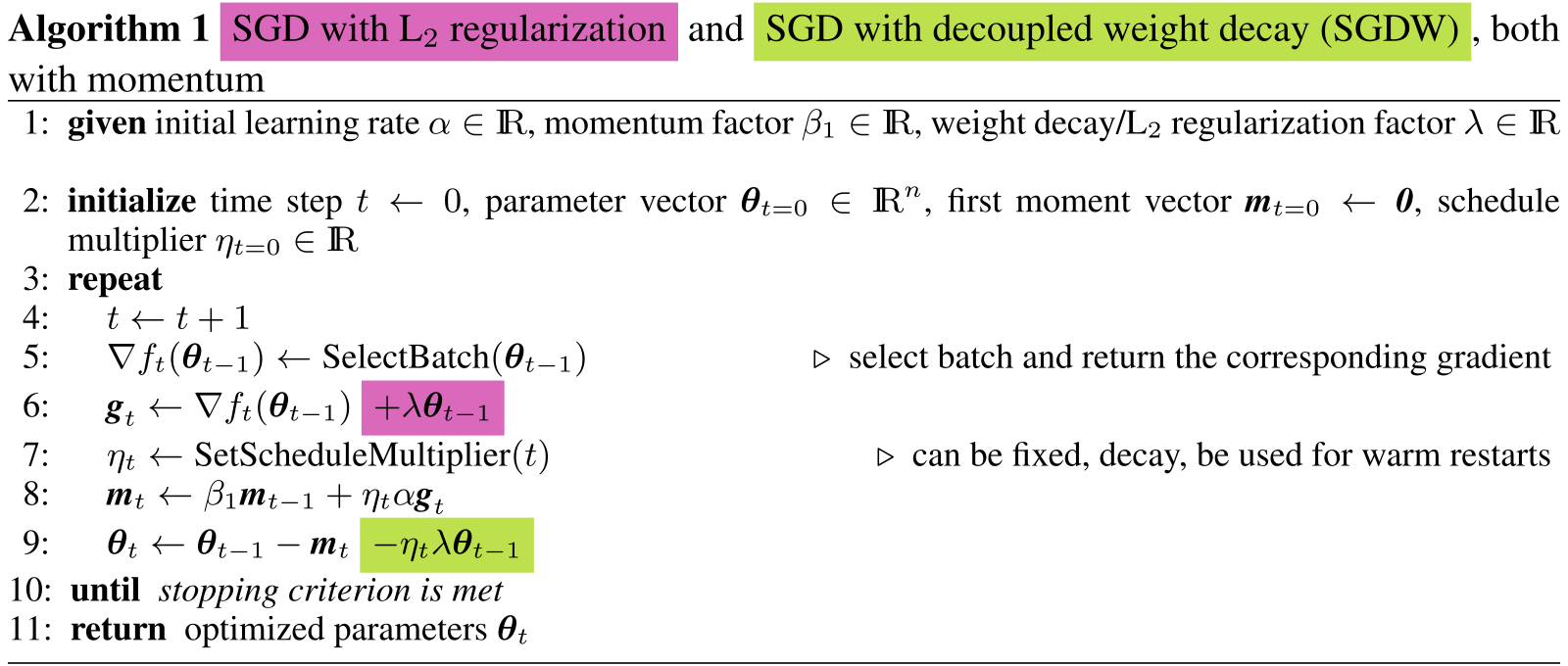
Accessible original algorithm markup (pink and green terms are alternatives)
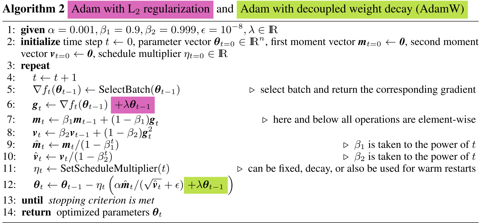
Accessible original algorithm markup (pink and green terms are alternatives)
Equation 2
| (2) |
3 Justification of Decoupled Weight Decay via a View of Adaptive Gradient Methods as Bayesian Filtering
The Bayesian-filtering interpretation is attributed to Aitchison’s subsequent analysis [Aitchison, 2018]. Under a Gaussian transition model and an approximate conjugate likelihood, posterior uncertainty preconditions the mini-batch gradient. A transition mean (I−A)θ with A=λI supplies parameter shrinkage separately from that gradient update. This motivates decoupled decay within the assumed filtering model; it is not a proof that AdamW must generalize better for arbitrary data and architectures. The paper distinguishes this contribution from its earlier empirical observation.
Equations 3–4
| (3) |
| (4) |
4 Experimental Validation
Experiments use Shake-Shake residual networks, batch size 128, and the data preprocessing and augmentation of the cited implementation. The main CIFAR-10 model is a 26 2x64d network with 11.6 million parameters; longer experiments use a 26 2x96d model with 25.6 million. ImageNet32x32 retains 1.2 million training examples and 1,000 classes at 32×32 resolution. These architecture, schedule, and budget choices matter when interpreting the optimizer comparisons.
4.1 Evaluating Decoupled Weight Decay With Different Learning Rate Schedules
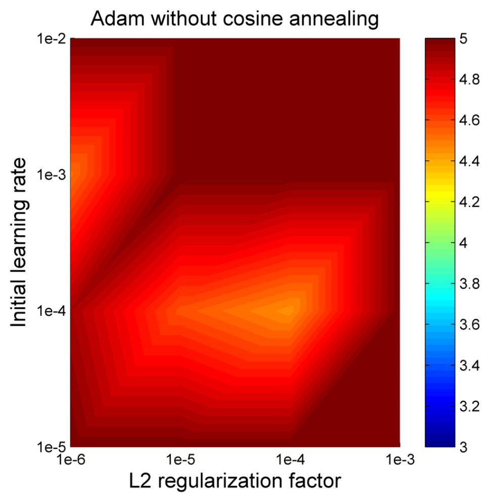
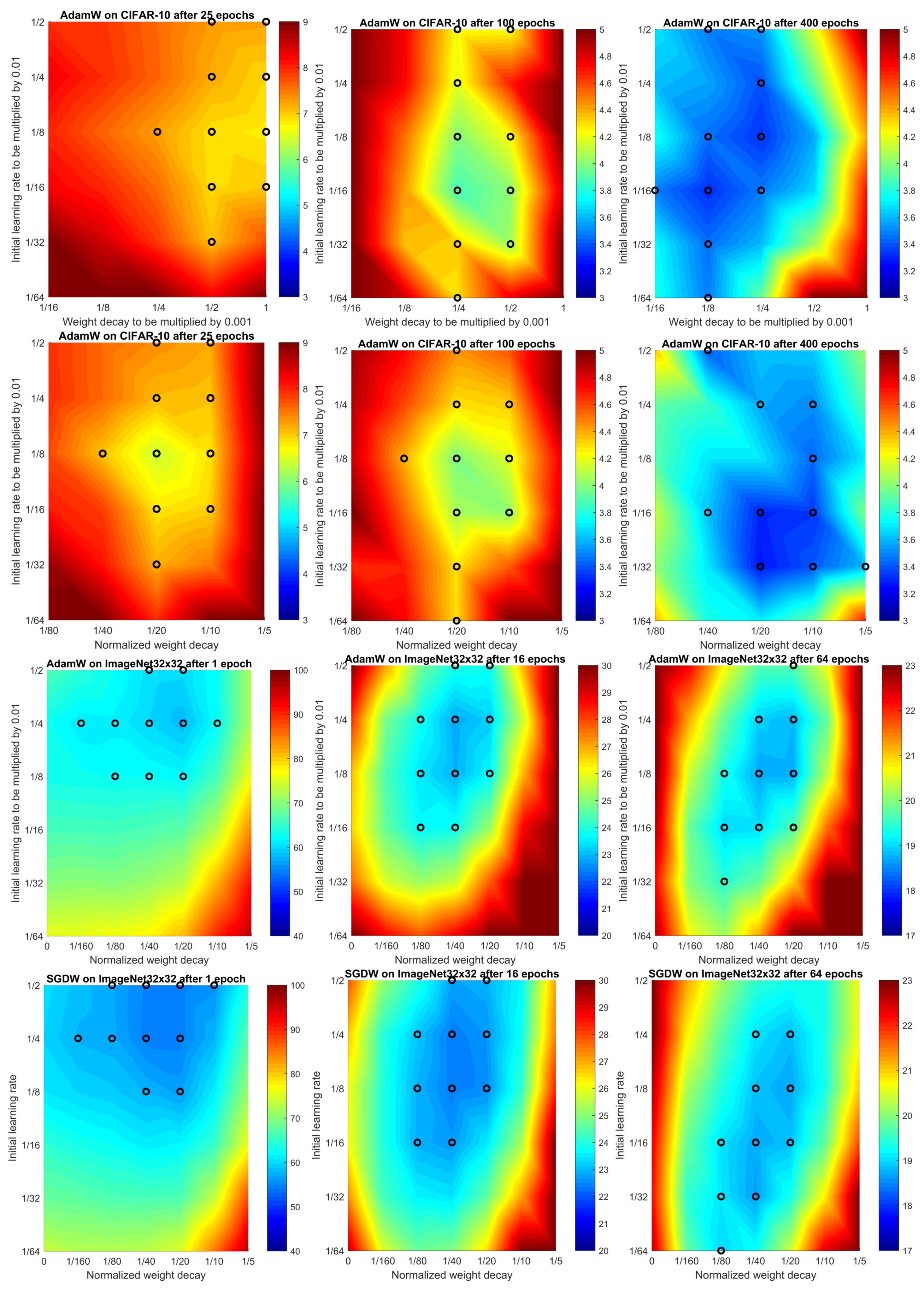
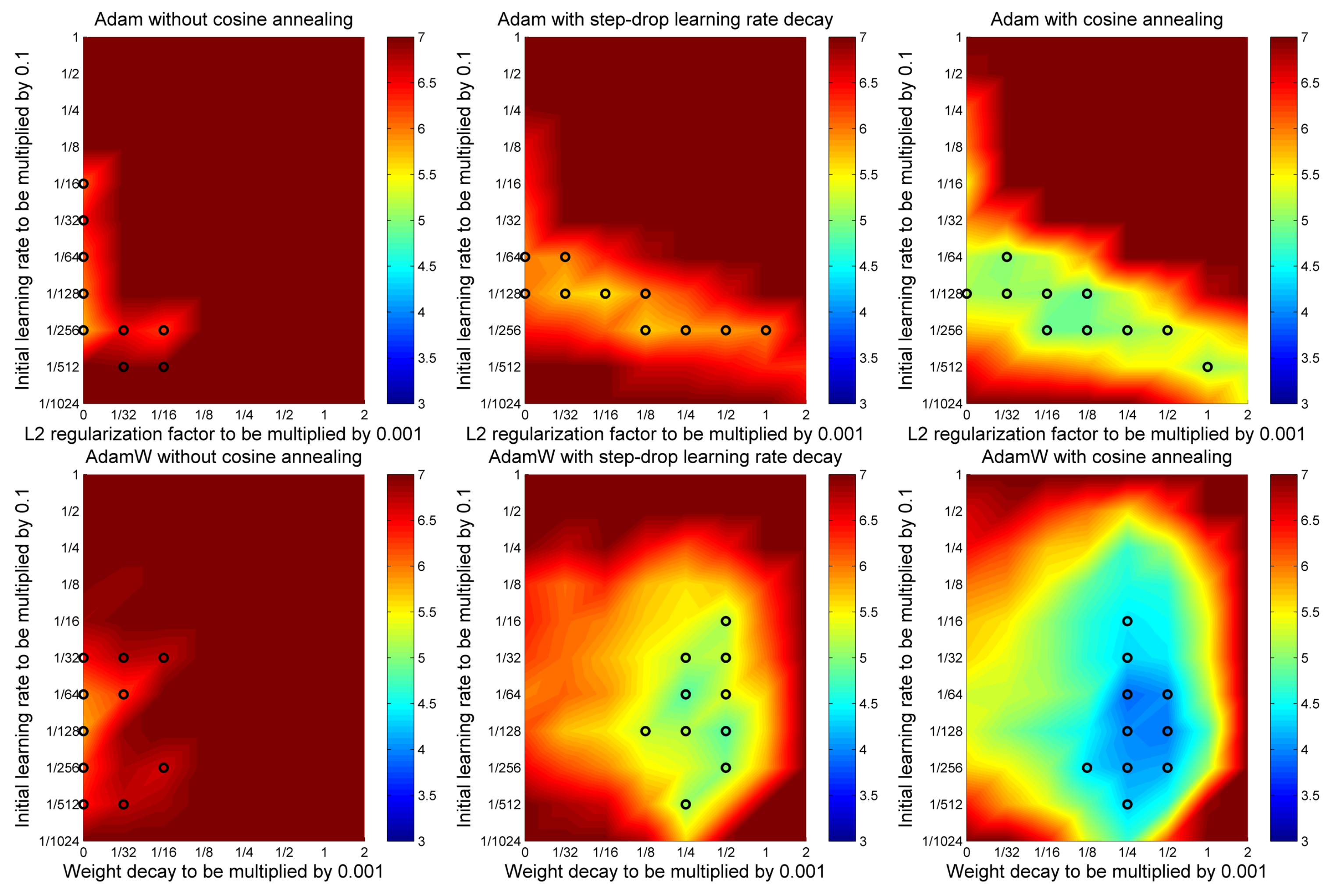
On CIFAR-10, a 100-epoch learning-rate/regularization grid compares constant rates, step reductions at epochs 30, 60, and 80, and cosine annealing. AdamW improves over Adam with L2 regularization in these grids, and cosine annealing gives the best results. Later experiments consequently use cosine schedules. Figure 1 preserves all six heat maps and their separately evaluated settings.
4.2 Decoupling the Weight Decay and Initial Learning Rate Parameters
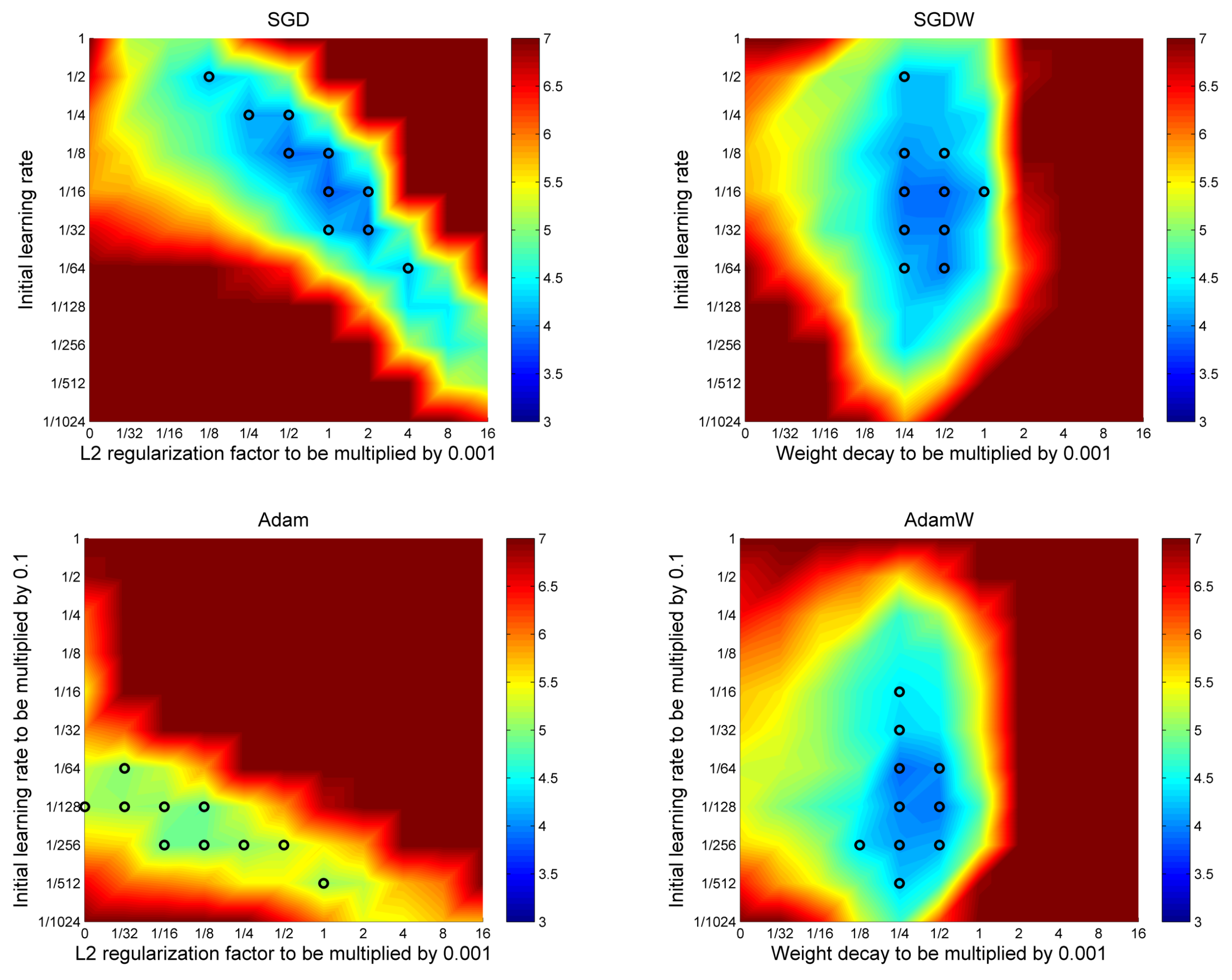
Figure 2 compares SGD and Adam with either L2 regularization or decoupled decay. The favorable regions are more nearly separable in learning-rate and decay coordinates for SGDW and AdamW, simplifying tuning in these experiments. This empirical geometry is stronger evidence for practical tuning behavior than the claim that all optimal settings are independent.
4.3 Better Generalization of AdamW
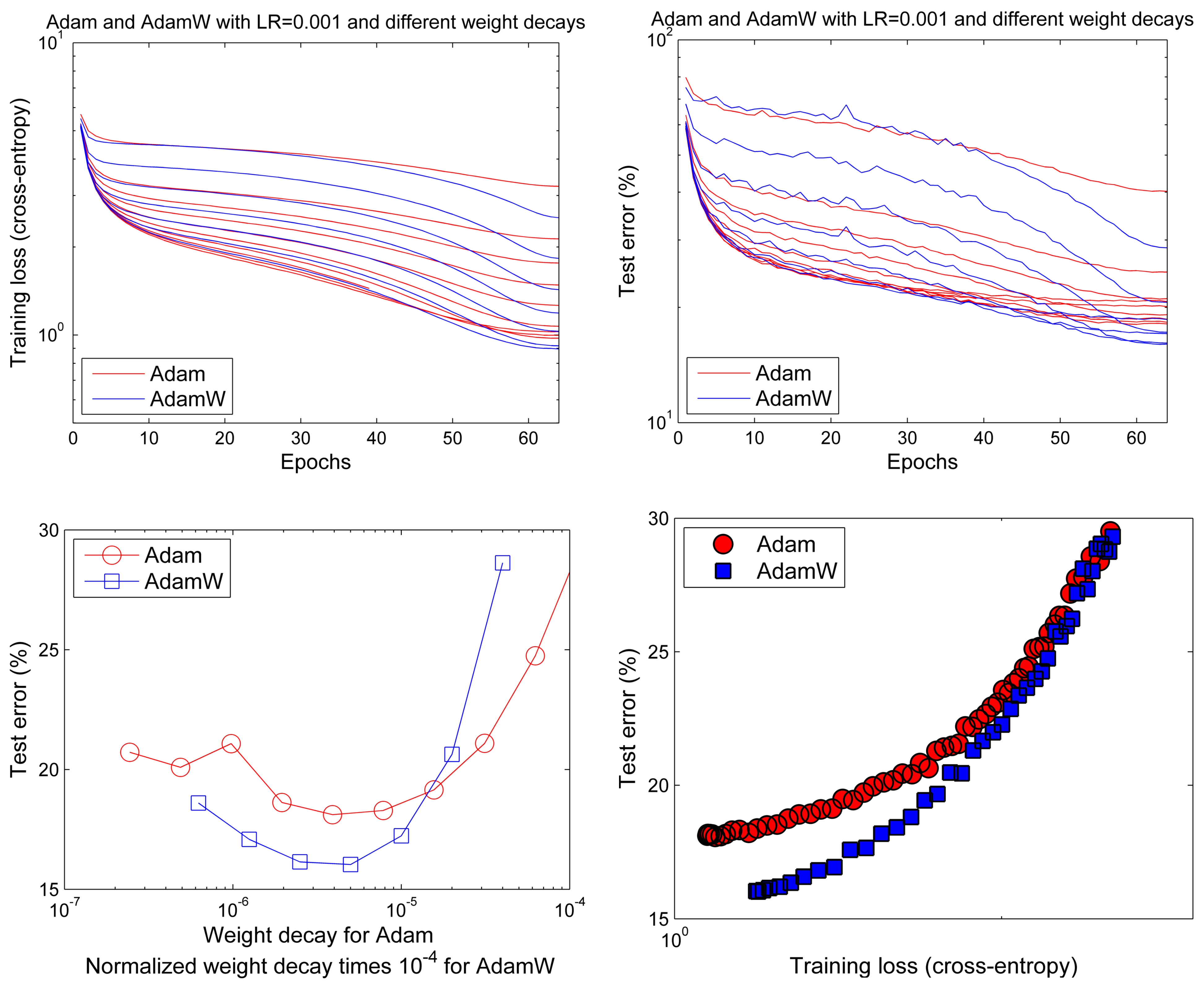
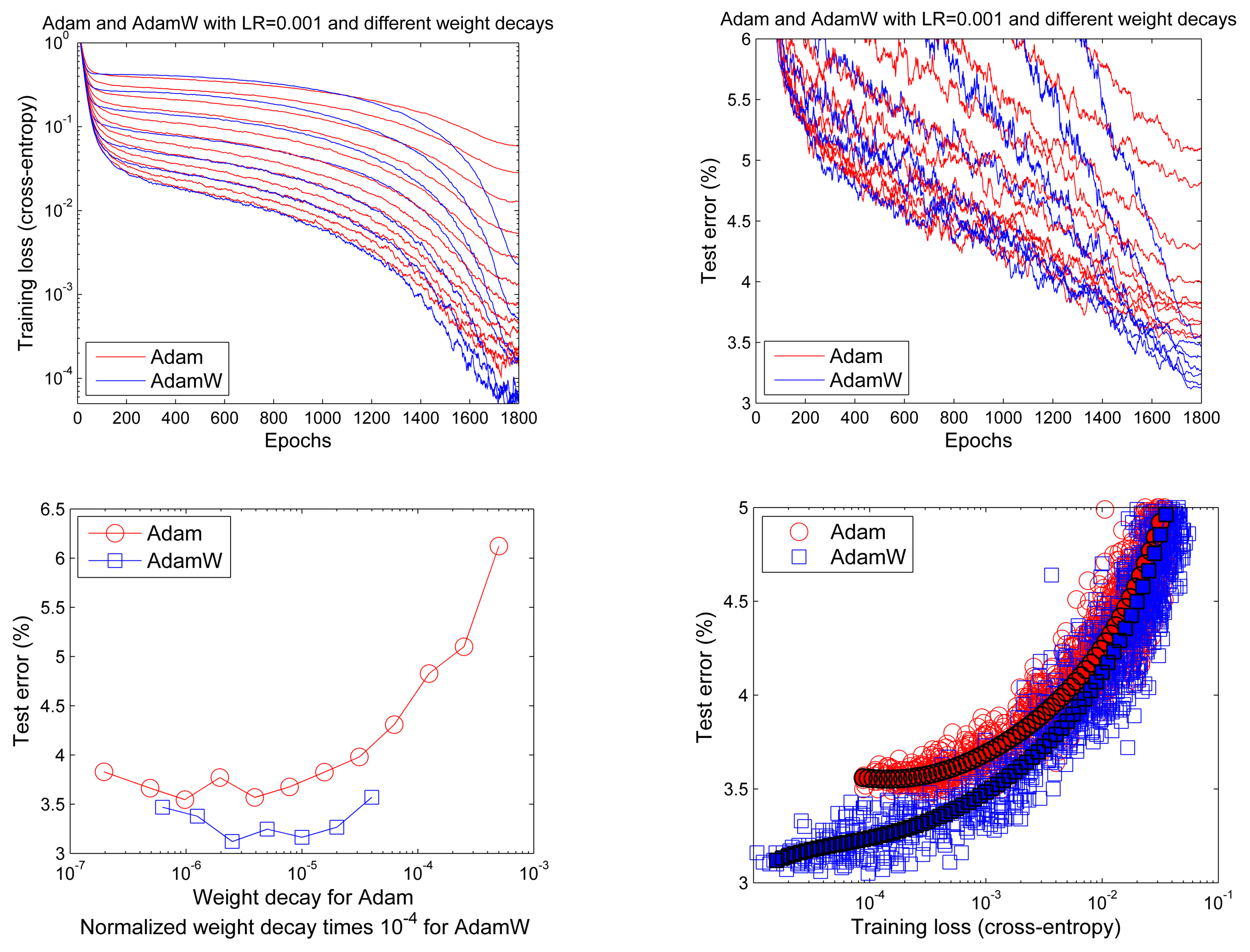
With learning rate 0.001, the larger CIFAR-10 network is trained for 1,800 epochs across 12 L2 settings and seven normalized-decay settings. AdamW achieves lower training loss and lower test error, including comparisons at similar training loss. The reported relative test-error improvement is about 15% on CIFAR-10 and ImageNet32x32 at this default learning rate. The plotted range of hyperparameters and training budgets defines that comparison; the result is not a benchmark-wide guarantee.
4.4 AdamWR with Warm Restarts for Better Anytime Performance
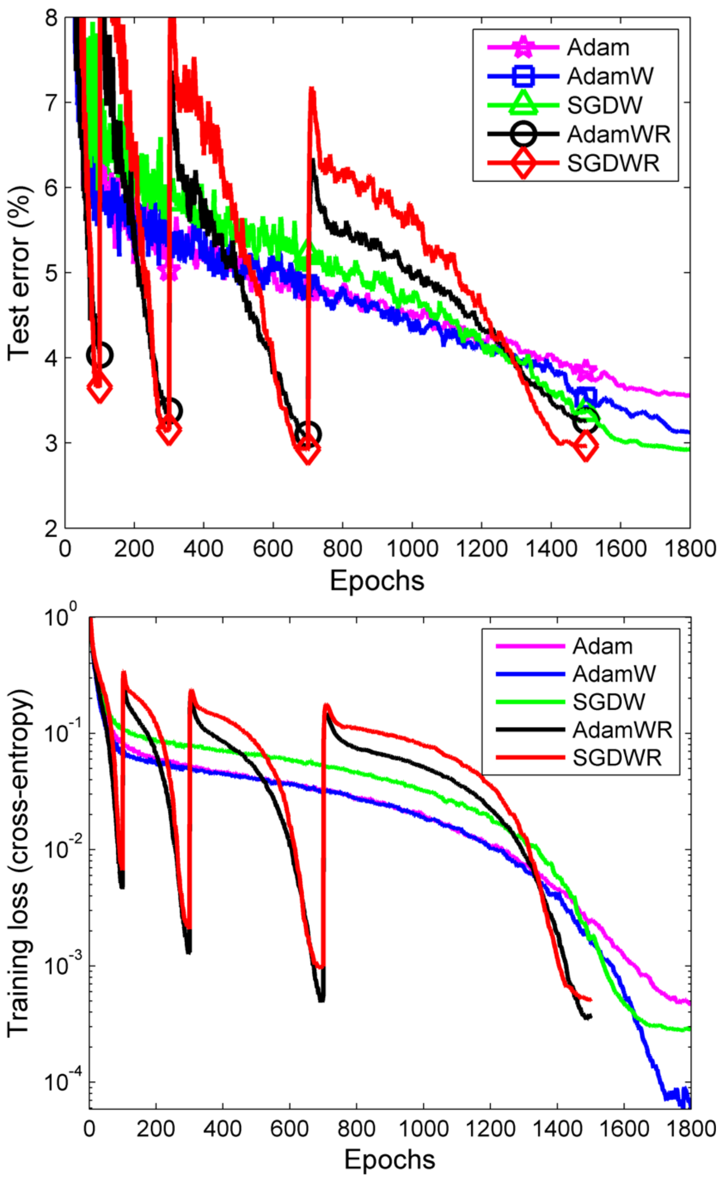
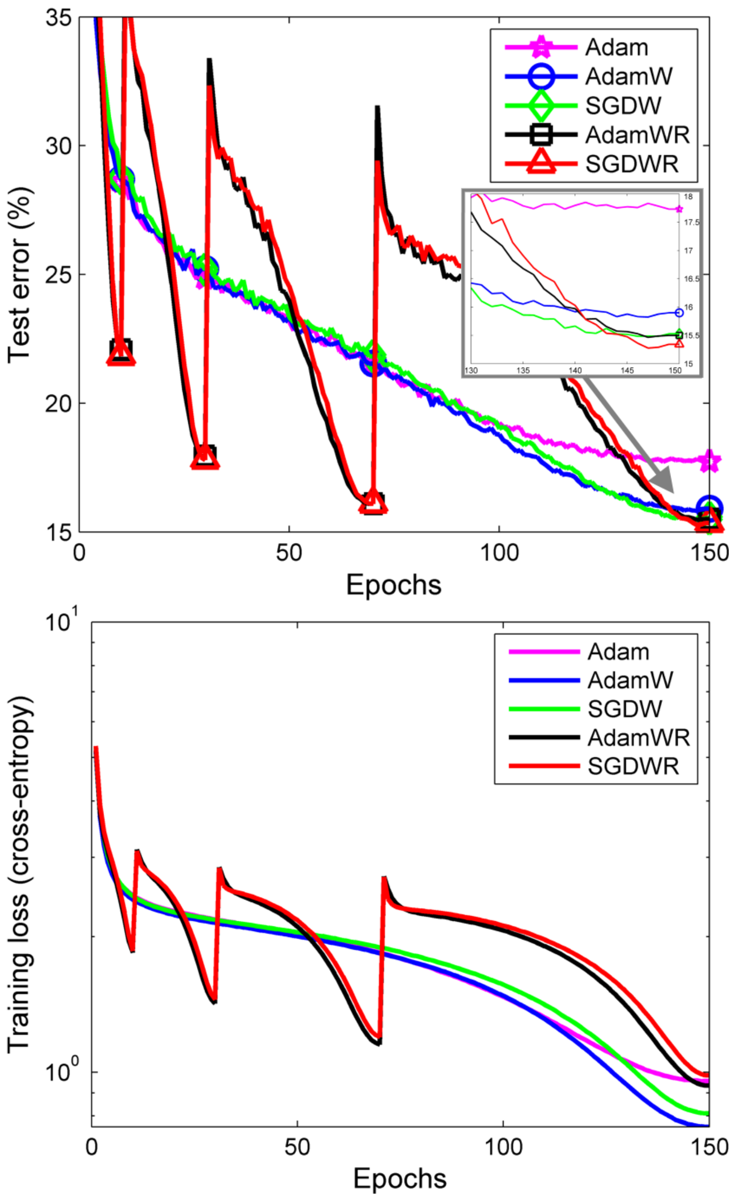
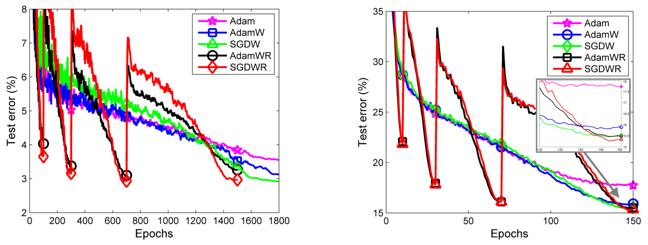
AdamWR combines decoupled decay with cosine warm restarts, analogous to SGDWR. Restarting the schedule keeps the learned weights and raises the learning-rate multiplier again. The first restart yields competitive checkpoints up to roughly ten times earlier in the illustrated learning curves, which is an anytime-performance statement rather than a tenfold reduction in the cost of each step. AdamWR closes much of the gap to SGDWR on CIFAR-10 and is comparable on ImageNet32x32; later checkpoints need not favor the same method.
4.5 Use of AdamW on other datasets and architectures
The authors discuss external applications rather than presenting a single controlled cross-domain benchmark. A face-analysis architecture reports faster predictions, but that system-level inference improvement cannot be attributed solely to its optimizer. In an EEG comparison supplied by collaborators, AdamW versus Adam reaches 73.68% versus 71.37% for Deep4Net and 72.04% versus 61.34% for a ResNet; the latter difference is reported significant. Language-model training and approximate natural-gradient work also use decoupled decay. These examples motivate broader study while retaining their separate architectures, data, and comparison conditions.
5 Conclusion and Future Work
The central recommendation is to distinguish direct parameter decay from an L2 loss penalty when implementing adaptive optimization. The image-classification experiments favor AdamW and show benefits from schedule design and decay normalization. Generality beyond these settings and adaptation to other optimizers remain open empirical questions. The fixed-preconditioner interpretation and the Bayesian model explain particular mechanisms without establishing universal generalization guarantees.
6 Acknowledgments
The authors acknowledge collaborators, reviewers, and compute assistance, and report support including the European Research Council and German Research Foundation. The complete original reference list is retained.
Appendix A Formal Analysis of Weight Decay vs L 2 Regularization
Appendix A proves the SGD identity by comparing coefficients of θ. For adaptive preconditioning, equality for all θ would require λI=αλ′Mₜ, impossible for the stipulated non-scalar Mₜ. For fixed diagonal scaling 1/s, a penalty λ′‖θ⊙√s‖²/2 yields a preconditioned penalty gradient λ′θ; setting λ′=λ/α reproduces direct decay. This last proof is the normalization used in the explanation above, and differs from the extra α printed in main-text Eq. 2. The derivations and their original notation remain available in full.
Equations 5–13
| (5) |
| (6) |
| (7) | |||||
| (8) |
| (9) | |||||
| (10) | |||||
| (11) |
| (12) | |||||
| (13) |
Appendix B Additional Practical Improvements of Adam
The following additions address how decay and learning-rate schedules change across training budgets; they are separate from the definition of AdamW.
B.1 Normalized Weight Decay
The heuristic sets λ=λ_norm√(b/(BT)), where b is batch size, B the number of training examples, and T the number of epochs. In a restarted run, T refers to the current cycle. This reduces the amount of retuning observed when budgets change and treats λ_norm as a normalized decay hyperparameter. The authors describe the evidence as preliminary and limited; this scaling is not derived as a universally optimal regularizer.
B.2 Adam with Cosine Annealing and Warm Restarts
Cosine annealing varies η between specified maximum and minimum values as a function of the fraction of the current cycle completed. Typical bounds are one and zero. At a warm restart the schedule is reset but the parameter vector is retained. Cycle lengths can grow by a fixed factor, here commonly two. This schedule is applied to both the gradient update and decoupled shrinkage as written in the algorithms.
Equations 14–15
| (14) |
| (15) |
Appendix C An Example Setting of the Schedule Multiplier
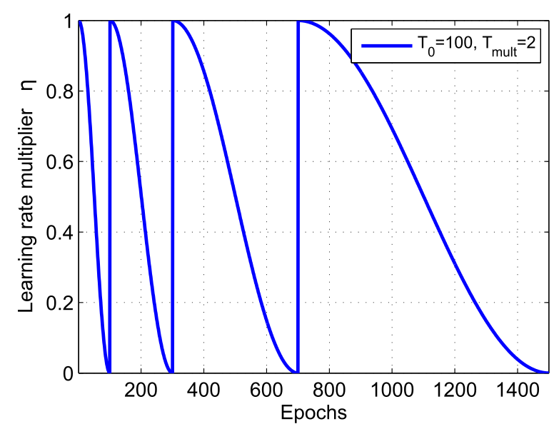
The example starts with 100 epochs and doubles cycle length, producing cycles of 100, 200, 400, and 800 epochs and checkpoints at 100, 300, 700, and 1,500 epochs. Supplementary Figure 1 shows the complete multiplier schedule.
Appendix D Additional Results
The supplementary results retain all six figures. A coarse 4×4 grid of fixed-rate Adam settings after 1,800 epochs reaches performance at best comparable to the earlier 100-epoch AdamW result, but the compared network sizes differ, so this is not a clean matched-compute speedup. The best raw decay decreases as the training budget grows. Normalized values around 0.025–0.05 work across the tested budgets and datasets, while an ImageNet32x32 epoch has about 24 times as many examples as a CIFAR-10 epoch; omitting the normalization can make decay about five times too large in that comparison. Supplementary Figure 4 repeats the loss/generalization analysis for ImageNet32x32, and Figures 5–6 add full training-loss curves to the restart comparisons. These observations support the proposed normalization in this experimental range, not an unrestricted scaling law.