The paper extends TP-GMM to learn two kinds of structure: when joint-space or task-space constraints matter, and which supplied priority hierarchy best explains demonstrations. Jacobian and null-space operators bring candidate behaviors into a common joint-space representation.
Experiments include COMAN bottle shaking and bimanual reaching, simulated Centauro priorities, and transfer to WALK-MAN. The method needs known kinematics, task set-points, and candidate hierarchies. Fusing hierarchies allows smooth trade-offs but does not guarantee every conflicting constraint.
Introduction
Dual-arm robots share joints, so simultaneous tasks can compete. End-effector goals alone may also miss important joint-level patterns, such as shoulder oscillation during shaking. The method uses demonstrated variability to identify the relevant space or priority structure instead of requiring fixed hand-tuned scalar weights.
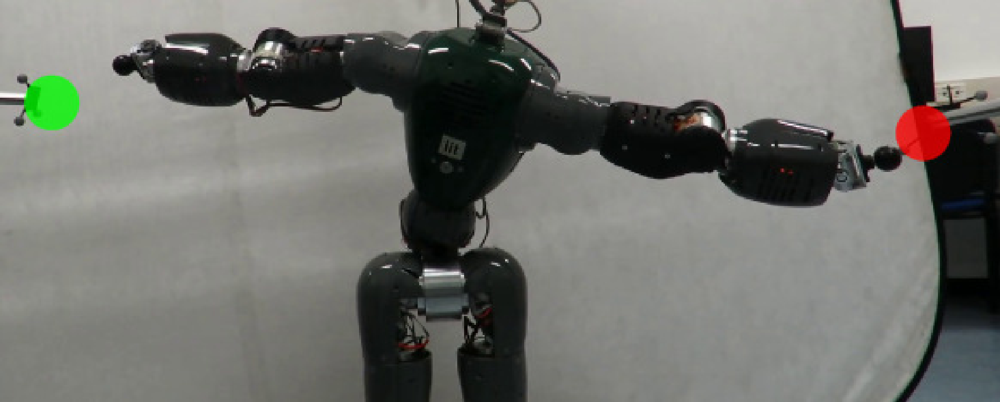
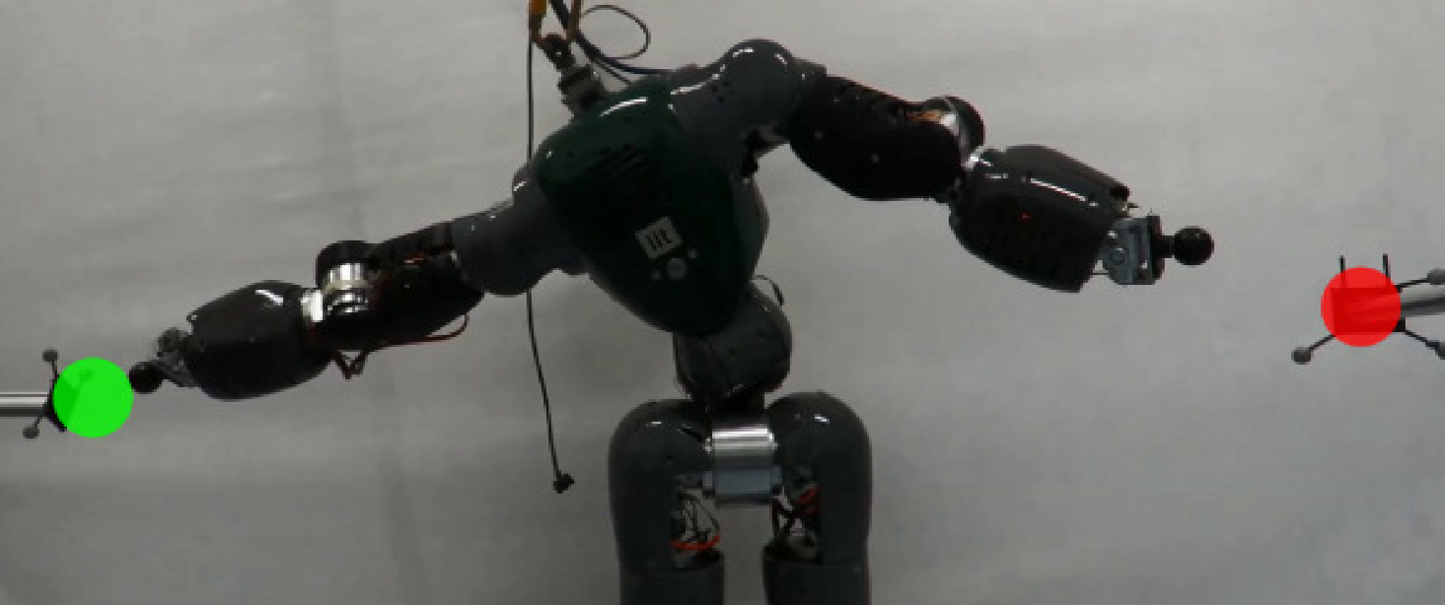
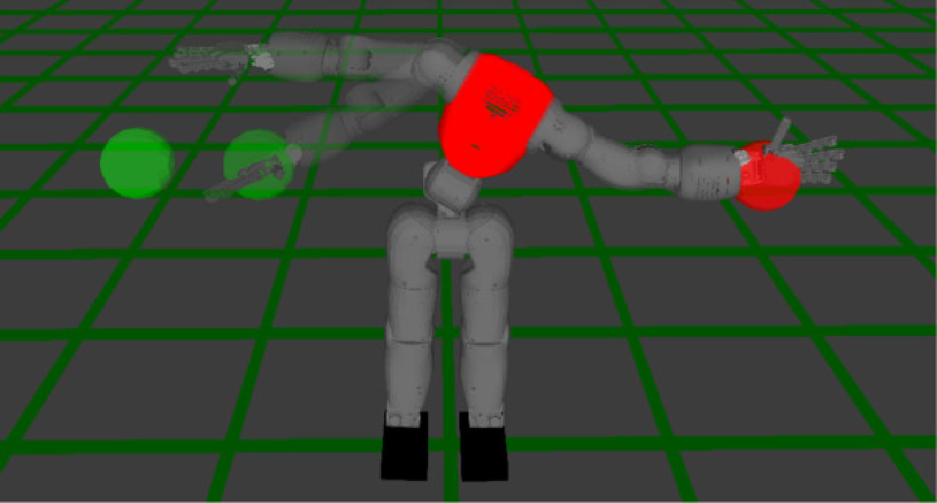
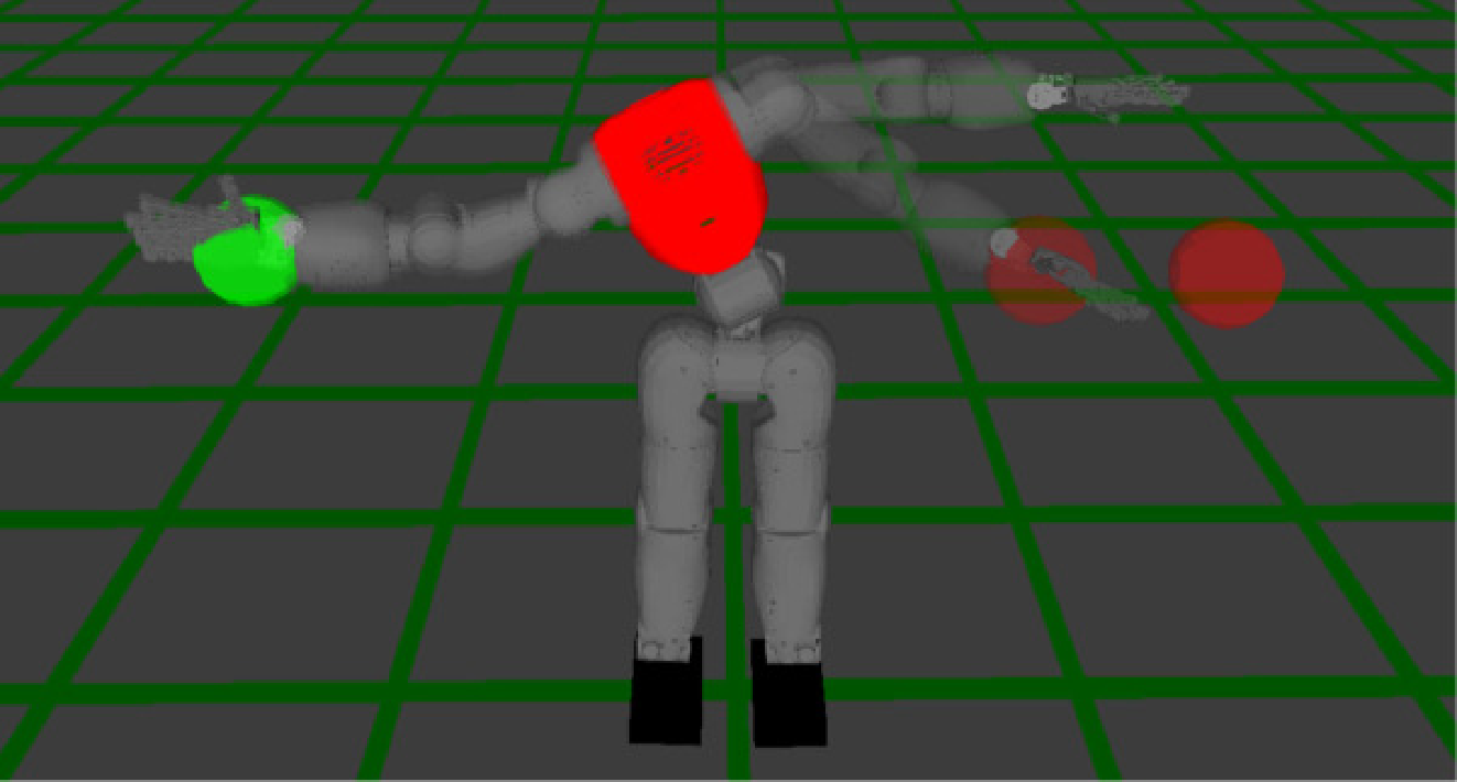
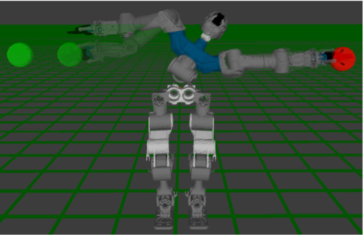
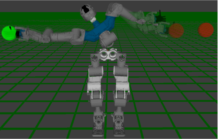
Fig. 1: The COMAN robot prioritizes the tracking of the left (resp. right) target, while doing its best to track the right (resp. left) one. This priority behavior was learned from demonstrations, using the approach proposed in Section V. Top: Reproduction with the model trained on left arm priority demonstrations. Bottom: Reproduction with the model trained on right arm priority demonstrations.
Related Work
Related work distinguishes learning bimanual motion, balancing task and joint spaces, and discovering priorities.
Learning bimanual skills
Many bimanual imitation methods encode coupled end-effector trajectories or forces. This captures operational-space coordination but can miss joint-space movement patterns and conflicts over shared joints.
Simultaneous learning of operational and configuration space constraints
Full covariance or precision matrices provide richer task weighting than scalars by expressing directional importance and correlations. The proposed Jacobian operators let the same probabilistic framework combine position, orientation, and configuration constraints.
Learning task prioritization
Strict hierarchies protect a high-priority task by projecting others into its null space. Soft weighting permits compromise and smoother transitions. The paper learns distributions over candidate strict-hierarchy solutions, then fuses those solutions.
1 Learning approaches based on strict hierarchies
Earlier methods learn null-space policies, constraints, or task stacks under various assumptions. Here demonstrations include task references and known kinematics, and the candidate hierarchy set is supplied in advance. Statistical consistency identifies the demonstrated structure; multiple Gaussian components can represent input-dependent priorities.
TABLE I: Contributions of our approach with respect to previous works on task priority learning.
2 Approaches related to soft weighting of tasks
Optimization-based weighting needs a fitness function, whereas demonstration-based methods infer importance from variation. Probabilistic prioritization of ProMPs learns task accuracy but does not identify the same strict-hierarchy candidates studied here. [36]
Task-Parameterized Gaussian Mixture Models
TP-GMM represents demonstrations from several task-dependent subspaces and recombines their local distributions when task parameters change.
Overview and nomenclature
Task parameters are affine operators mapping local Gaussian models into a common space. Earlier versions used object coordinate frames. This work broadens those operators to Jacobian projections and candidate task hierarchies. Table II defines the notation used throughout.
Mean and covariance of Gaussian for task parameter
Mixing coefficient of Gaussian
Number of demonstrations
Number of datapoints in demonstration
Total number of datapoints in a demonstration dataset
Dimension of datapoints
Datapoint at time
Demonstration dataset
Robot
Cartesian position of left and right end-effectors
Orientation of left and right end-effectors as unit quaternions
Orientation of left and right end-effectors as rotation matrices
Number of robot joints
Joint angles of left and right arms
Jacobian matrices of left and right arms
Priority operator (the task on the operator left has priority over the one on the right)
TABLE II: Summary of the notation.
Model estimation
Each demonstration is transformed into a local dataset for each candidate subspace. Expectation maximization fits shared mixture weights and local means and covariances. Variability in each subspace encodes how consistently that constraint was demonstrated.
Gaussian Mixture Regression
For a new situation, affine transformations map local Gaussian components into a common space. Their product combines means according to precision. GMR then conditions on an input such as time to generate a reference trajectory distribution. Task parameters may change during reproduction.
Equations 1–3
(1)
(2)
(3)
Learning operational and configuration space constraints simultaneously
Encoding demonstrations in both joint and operational spaces lets the model emphasize the space with more consistent demonstrated constraints at each phase. Jacobian-based affine maps bring task-space distributions into joint space before fusion.
Jacobian-based task parameters for position constraints
Locally integrated inverse differential kinematics expresses joint references as affine functions of desired Cartesian position. Gaussian transformation rules then project position means and covariances into joint space. Additional rotation and translation terms support positions specified relative to objects. The derivation assumes the relevant pseudoinverse is well defined or suitably regularized.
Equations 4–7
(4)
(5)
(6)
(7)
TABLE III: Summary of task parameters as candidate projection operators
Configuration space constraints:
Absolute position constraints:
Relative position constraints:
Absolute orientation constraints:
Relative orientation constraints:
Task parameters for orientation
Unit-quaternion multiplication provides an analogous local linear map for orientation constraints. Combining this with the angular Jacobian projects orientation distributions into joint references. This is an approximation of quaternion geometry; the discussion proposes manifold-based formulations as a future refinement. Algorithm 1 preserves the complete learning and synthesis procedure.
Equations 8–12
(8)
(9)
(10)
(11)
(12)
Algorithm 1 Simultaneously learning constraints in operational and configuration spaces
1:Initialization
2:Select candidate projection operators from Table III based on the task at hand
•
Canonical operator , , for encoding configuration space constraints
•
Operational space operators, for absolute or relative position/orientation constraints in operational space
3:Collect demonstrations and compute the local datasets according to the chosen operators
10: Use as joint references for the robot controller
11:endfor
Task parameters for configuration space constraints
Joint-space demonstrations use the identity projection. Their Gaussian distribution is fused with the projected position and orientation constraints, allowing the same model to change emphasis across movement phases.
Experiment: bimanual shaking skill
Ten approximately thirteen-second simulated demonstrations teach COMAN to reach for a bottle and shake it with its shoulders. Data are temporally aligned; a ten-component model uses one bottle-relative operational operator and one joint-space operator. The setup assumes a successful grasp with fixed contact points.
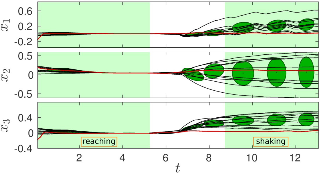
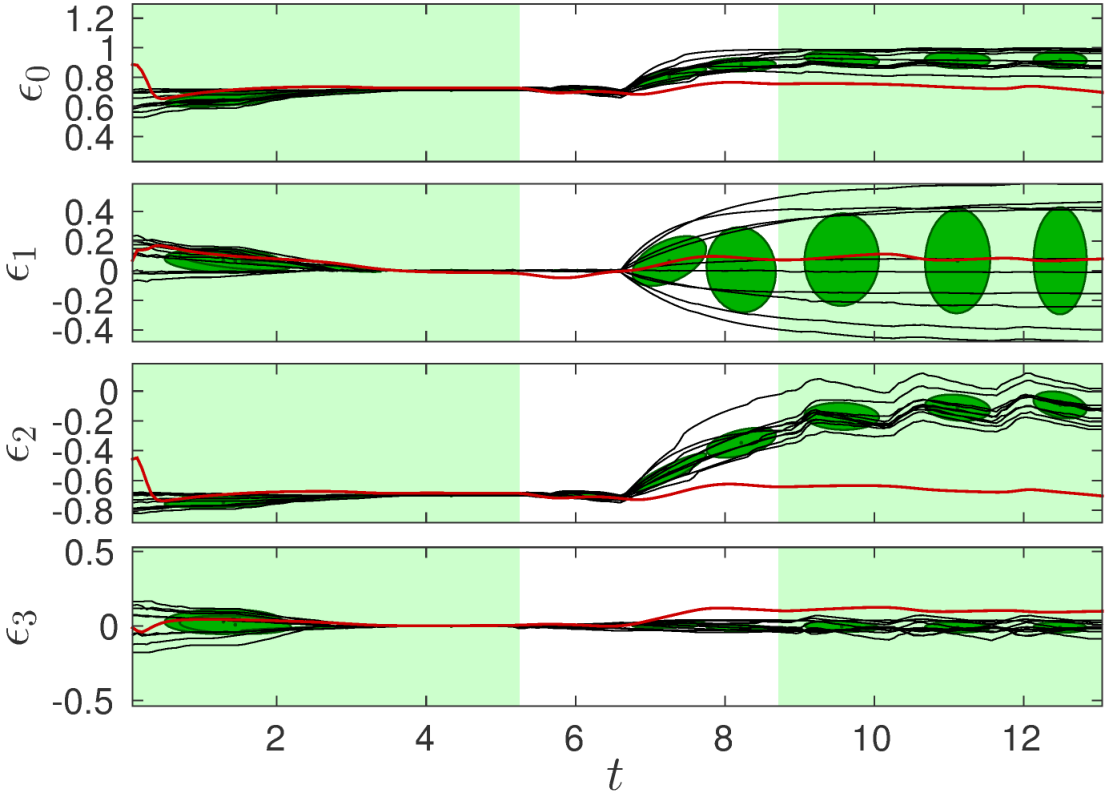
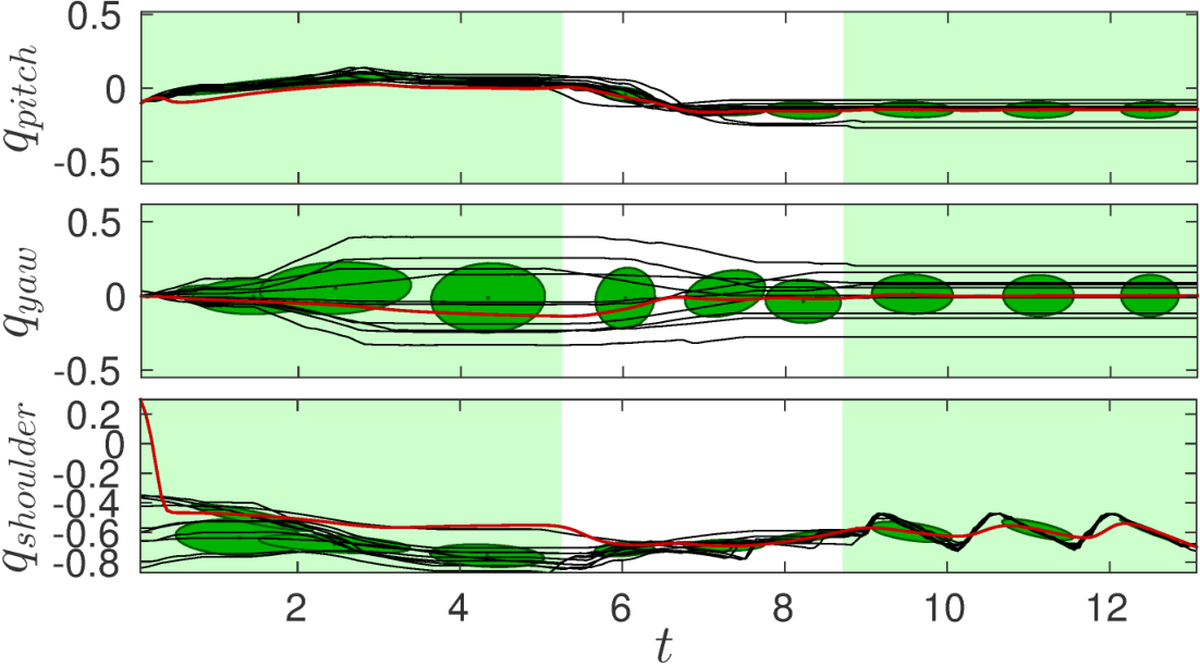
Low variation in bottle-relative pose dominates reaching, while consistent shoulder oscillation dominates shaking. A physical COMAN reproduction uses optical object tracking and joint-position control. This demonstrates switching between relevant spaces rather than learning grasp reliability from raw sensory data.
Equations 13–16
(13)
(14)
(15)
(16)
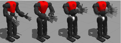
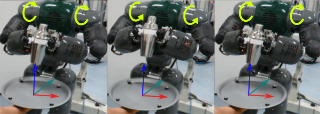
Fig. 2: The COMAN robot performs the bimanual shaking task in simulation. First: The robot is in a neutral starting pose. Second: Reaching for the bottle and grasping it. Third: Bringing the bottle close to the torso. Fourth: Shaking movement executed through rhythmic oscillations of both shoulder joints.
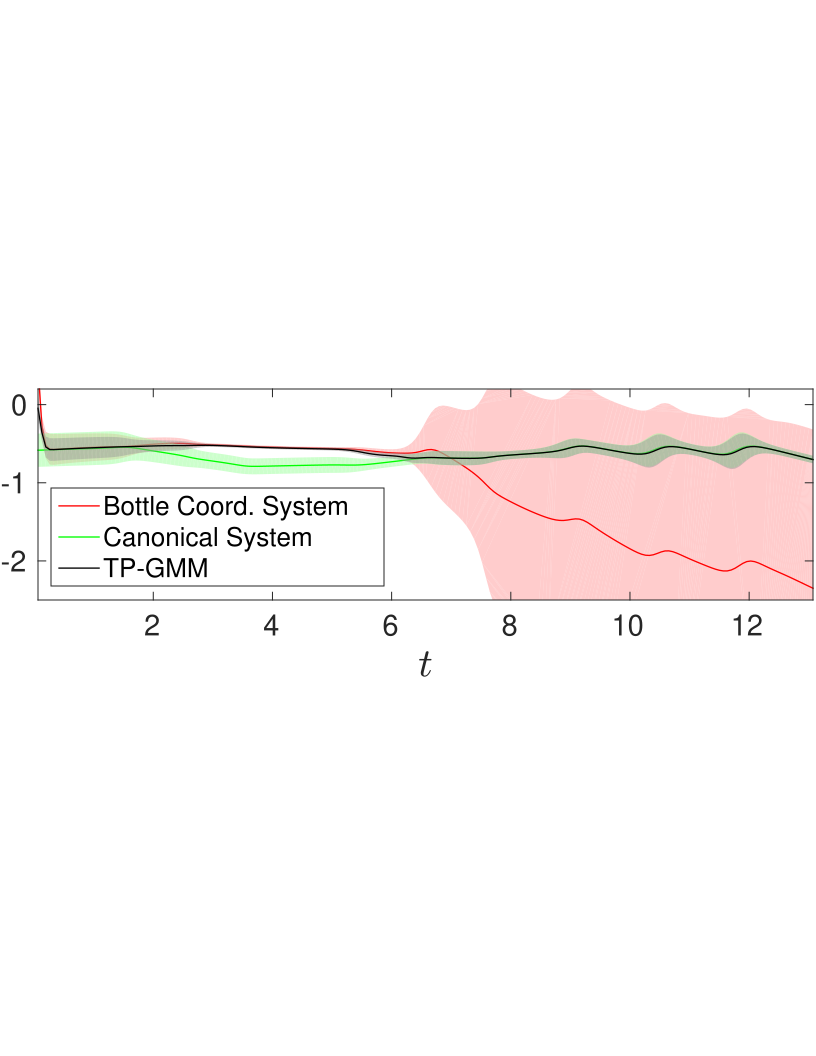
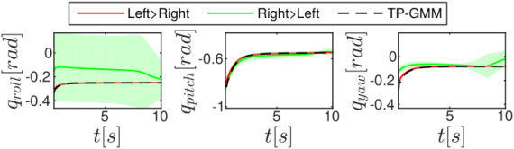
Fig. 3: Reproduction of the shaking task in the real COMAN robot. Top: Snapshots of the reaching part of the movement, defined by constraints in operational space. The robot gradually reaches for the object, which is tracked using an optical system. Bottom: Shaking part of the movement, defined by constraints in configuration space. The robot performs the shaking through rhythmic motions of the shoulders, moving the shaker up and down repeatedly.Fig. 4: Left end-effector position (in meters) with respect to the initial bottle coordinate system (prior to the grasp). Black lines represent demonstrations while the red line represents one reproduction of the movement. Ellipses depict the Gaussian components of the model (isocontour of one standard deviation). The shaded areas mark the duration of the reaching and shaking phases. Notice the low variability in position at the end of the reaching movement.Fig. 5: Left end-effector orientation (as a unit quaternion) with respect to the initial bottle coordinate system (prior to the grasp). Notice the low variability in orientation at the end of the reaching movement.Fig. 6: Waist joints (pitch and yaw) and shoulder joint of the left arm (in radians). Notice the low variability of the shoulder joint during the shaking part of the movement (second shaded area) and how the model captures the shaking pattern encoded in this joint.Fig. 7: Shoulder joint angle estimation (radians) from each space (red and green) and the resulting reference after TP-GMM (black). Each estimate has an associated mean (solid line) and variance (light color envelope), learned from demonstrations and synthesized during reproduction.
Learning task prioritization hierarchies from demonstrations
Hierarchy learning first identifies statistically consistent candidates, then uses their learned precision to combine velocity commands in new situations.
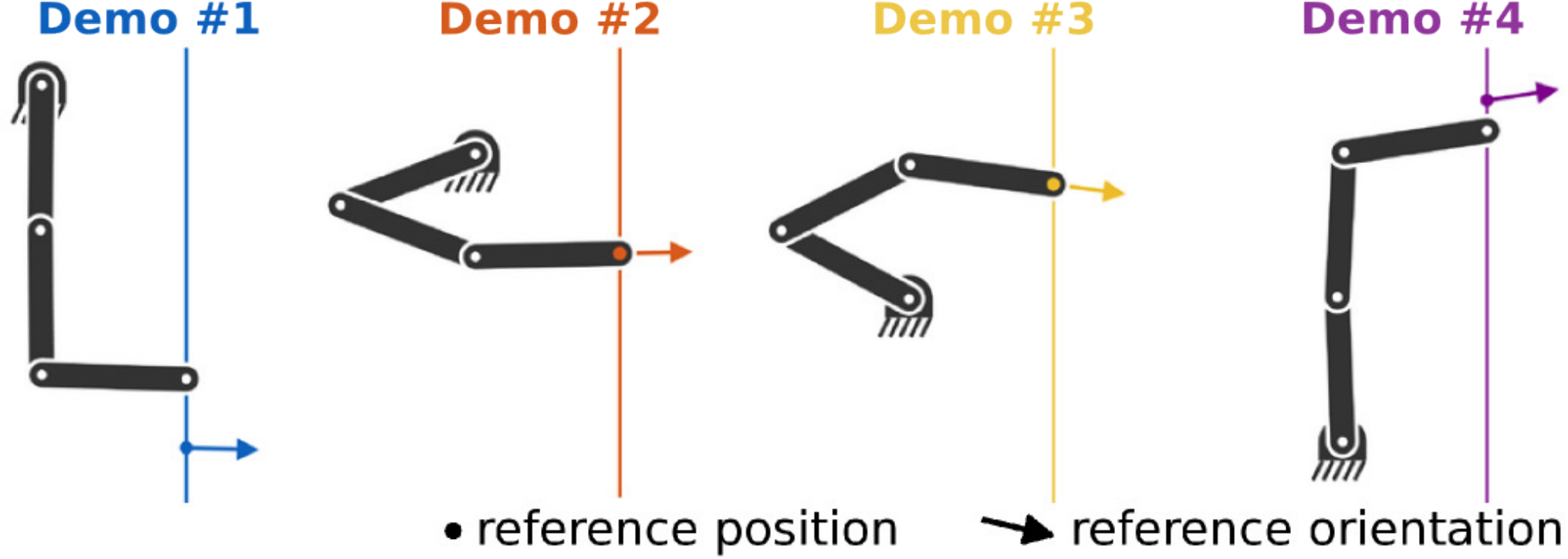
(a)Four demonstrations of priority on orientation. The robot only fulfills the two tasks when they are both achievable (demonstrations 2 and 3). When they are incompatible, orientation is prioritized (demonstrations 1 and 4).
(b)Four demonstrations of priority on position. Once the two tasks become incompatible the robot prioritizes position tracking (demonstrations 1 and 4).
Fig. 8: Planar robot tracking an orientation (arrow) and a vertical position (dot) along a line, with different priorities.
Identifying priority hierarchies from demonstrations
For each candidate hierarchy, Jacobians and null-space projectors map the known task-error commands into predicted operational motion. Demonstrations are more consistent under the hierarchy that generated them. Local Gaussian models encode that consistency.
The procedure generalizes to several tasks but assumes a known kinematic model, available task Jacobians, and known task set-points. It identifies among supplied candidates rather than discovering arbitrary tasks from unstructured observation.
Equations 17–20
(17)
(18)
(19)
(20)
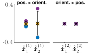
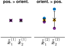
(a)Demonstrated priority on orientation (see Figure 8(a)).
(b)Demonstrated priority on position (see Figure 8(b)).
Fig. 9: Operational space velocities generated by each candidate hierarchy for the configurations of the robot in Figure 8. Each colored point corresponds to a demonstration with the same color in Figure 8. The ‘’ represents the mean of the datapoints, while the bars depict one standard deviation. Equation 21
(21)
Movement synthesis: fusion of strict hierarchies
At execution, GMR predicts covariance for each candidate hierarchy. Mapping it into joint space gives a precision matrix; a weighted least-squares solution fuses the candidate joint velocities. The result can be sent to a velocity controller or integrated for position control. Algorithm 2 retains all initialization, fitting, and synthesis steps.
Equations 22–25
(22)
(23)
(24)
(25)
Algorithm 2 Learning task prioritization hierarchies from demonstrations
1:Initialization
2:Select a set of potentially relevant candidate hierarchies
Experiment: Fusion of hierarchies and behavior during transitions
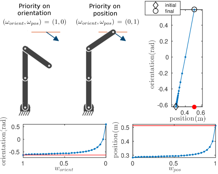
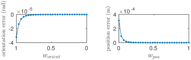
A planar test manually changes hierarchy weights to examine transitions before learning them. Incompatible position and orientation goals produce a smooth compromise as weights vary. When both goals are reachable, the demonstrated test maintains both after convergence. These examples illustrate behavior, not a universal convergence proof for arbitrary conflicting tasks.
Fig. 10: End-effector behavior for varying hierarchy weights. Top-left: Planar robot fulfilling the two tasks separately. Top-right: End-effector state in the position-orientation space for the considered weights (blue line). Bottom: End-effector orientation and vertical position as weights vary. Note the inverted scales on the horizontal axes (the experiment starts with and ends with ). Red lines and point indicate the references.Fig. 11: Performance of the robot in tracking position and orientation references with varying weights when both tasks can be achieved.
Experiment: Learning priorities with the COMAN robot
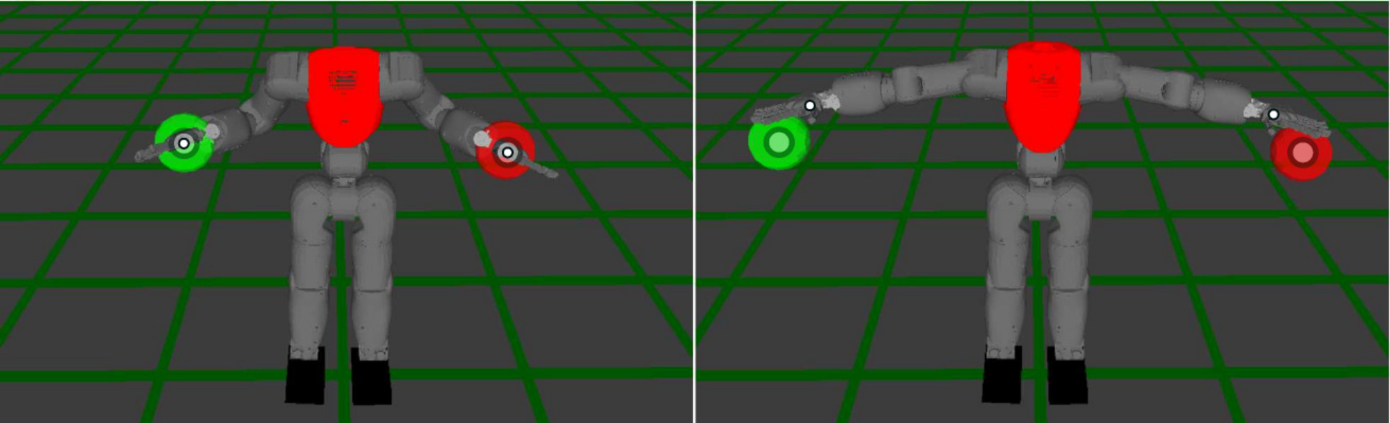
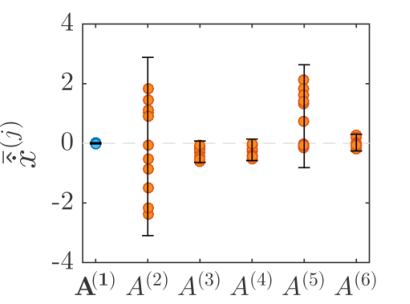
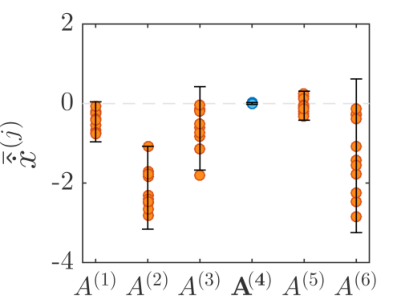
COMAN’s shared waist joints create conflicts between left- and right-hand reaching. Two candidate hierarchies and one Gaussian encode a constant priority learned from simulated controller demonstrations. Physical tests use optically tracked targets and reproduce the preferred arm’s tracking while attempting the secondary task.
Reported per-step computation averages 1.15 milliseconds in MATLAB on the specified laptop. Low variance under the demonstrated hierarchy gives it greater precision in the combined controller.
Fig. 12: Illustration of the waist joint prioritization problem. Left: Both targets are within the reachable workspace of both arms, so the robot can successfully reach the centers of the spheres with the palm of its hands. Right: References become simultaneously unreachable, so the robot cannot reach any of the two. The small circles depict the tool center point of each arm, while the large circles represent the centers of the references.
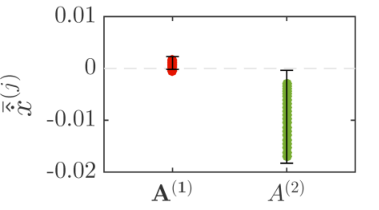
(a)Demonstrated left arm priority.
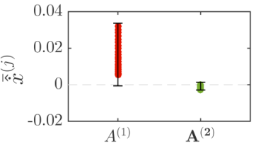
(b)Demonstrated right arm priority.
Fig. 13: Task space velocities generated by each candidate hierarchy given the demonstration data. Each entry contains the means of several observations , computed across the dimensions of the tasks. The error bars correspond to two standard deviations of the data. Note the low variability in the datapoints corresponding to the demonstrated hierarchies.Equations 26–27
(26)
(27)
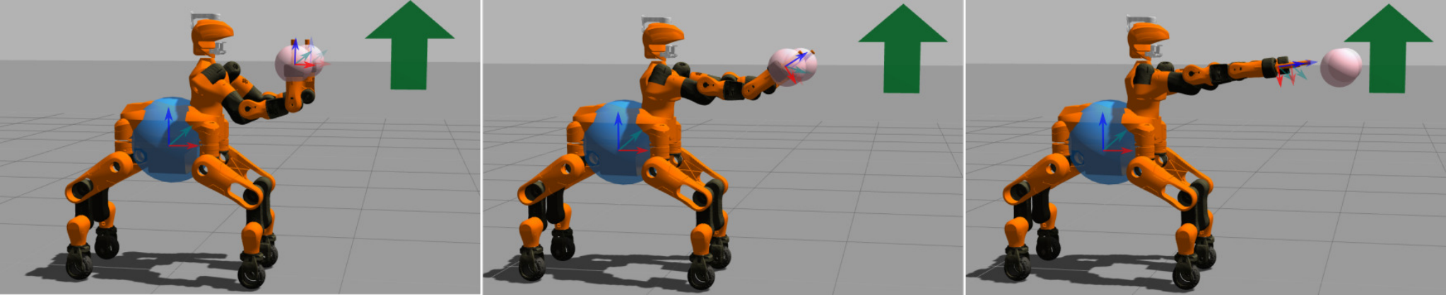
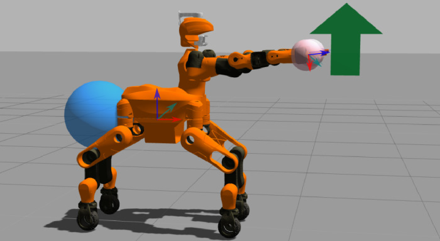
Fig. 14: Movement synthesis using the learned left and right arm priority models. Left: The left reference is always tracked, while the right reference is only tracked when reachable. Right: The right reference is prioritized.Fig. 15: Waist joint angles given by each candidate hierarchy. The envelope around the lines represents one standard deviation of the variance encoded in each hierarchy. TP-GMM extracts the solution with the lowest variability. Fig. 16: The Centauro robot tracks different references, prioritizing (by decreasing order of importance) base position, end-effector positions and end-effector orientations. The blue and pink spheres represent the desired base and end-effectors positions, while the arrow denotes the desired end-effector pointing direction. Left: All tasks can be fulfilled. Center: The pelvis reference is moved backwards, thus the robot performs the orientation task as best as it can but not completely. Right: The end-effector position references are moved forward and both end-effector position and orientation are now only partially fulfilled.
(a)Demonstrated: .
(b)Demonstrated: .
Fig. 17: Datasets from Centauro priority demonstrations. Each entry contains 12 points (the means of for each demonstration).Fig. 18: In this example, the Centauro robot prioritizes end-effector positions, followed by the position of the base and, finally, the end-effector orientations.
Experiment: Learning priorities with more than two tasks
Centauro is evaluated in simulation with wheel-only locomotion, controlling nineteen joints. Three task groups—base position, hand positions, and hand orientations—produce six candidate orderings. Twelve demonstrations teach one ordering, and twelve more separately teach another.
Both demonstrated orderings are identified and reproduced with changed references. The unoptimized implementation averages 7.35 milliseconds per control cycle on different hardware; this is not a directly controlled speed comparison with COMAN.
Experiment: Transferring task priorities between robots
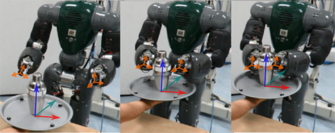
Priority models learned on COMAN transfer to the kinematically different WALK-MAN model. Both share the relevant operational-space dimensions and the structure in which waist joints affect both arms. The experiment supports transfer within that correspondence, while learning priorities directly from human vision remains a proposed extension.
Fig. 19: Movement synthesis with the WALK-MAN robot using the left and right priority models that were learned with COMAN.
Discussion
The discussion separates limitations of task-space fusion from limitations of hierarchy identification.
Learning operational and configuration space constraints
Demonstrations must vary enough to reveal which constraints matter. Poorly varied examples can mislead the model. Quaternion handling is approximate, and conflicting constraints are fused without explicitly deciding whether the compromise is acceptable. Interactive teaching and conflict detection are future directions.
Learning task prioritization hierarchies
Candidate hierarchies and task set-points must be specified. Too many candidates increase data requirements, and moving set-points complicate demonstration collection. Separately teaching individual tasks and their priority relationships is suggested as a way to reduce that burden.
Conclusions and Future Work
The framework combines operational and joint-space constraints and learns priority behavior among supplied hierarchies. Evidence covers the reported humanoid and simulated mobile-manipulation scenarios. Torque control, optimization-based refinement, and more general whole-body contact priorities remain future work.
Author information
The source includes portraits of the four authors. Affiliations below are those stated in the paper.
João Silvério — Istituto Italiano di Tecnologia, as listed in the paper.
Sylvain Calinon — Idiap Research Institute, as listed in the paper.
Leonel Rozo — Istituto Italiano di Tecnologia, as listed in the paper.
Darwin G. Caldwell — Istituto Italiano di Tecnologia, as listed in the paper.
Earlier-manuscript Appendix A: Unit quaternions
These mathematical appendices come from the 2017 arXiv v1 manuscript. The current paper moves them to an external supplement whose original link is unavailable. Their equation numbers belong to the earlier manuscript.
A unit quaternion has a scalar part and a three-dimensional vector part, with unit norm. Conjugation negates the vector part. Quaternion multiplication composes rotations and is generally noncommutative. Left and right Hamilton matrices express that product as a matrix–vector operation; their respective actions commute. The original product and matrix formulas are preserved below.
Equations v1 28–v1 30
(v1 28)
(v1 29)
(v1 30)
Earlier-manuscript Appendix B: Linear orientation operators
The earlier derivation selects the vector part of the relative quaternion with a fixed matrix and rewrites quaternion multiplication using the right Hamilton matrix. Once the previous orientation is fixed, the next quaternion enters linearly. This supplies the local orientation operator used by TP-GMM.
The formulas use the paper’s discrete angular-velocity approximation, not an exact finite-rotation logarithm. The current main text explicitly uses an approximation sign; the earlier appendix also discusses quaternion logarithmic mappings as an alternative.
Equations v1 31–v1 34
(v1 31)
(v1 32)
(v1 33)
(v1 34)
46 references
[1]
C. Smith, Y. Karayiannidis, L. Nalpantidis, X. Gratal, P. Qi, D. V.
Dimarogonas, and D. Kragic, “Dual arm manipulation – a survey,”
Robotics and Autonomous Systems, vol. 60, no. 10, pp. 1340 – 1353,
2012.
[2]
A. G. Billard, S. Calinon, R. Dillmann, and S. Schaal, “Robot programming by
demonstration,” in Handbook of Robotics, B. Siciliano and O. Khatib,
Eds. Secaucus, NJ, USA: Springer,
2008, pp. 1371–1394.
[3]
A. Gams, B. Nemec, A. J. Ijspeert, and A. Ude, “Coupling movement primitives:
Interaction with the environment and bimanual tasks,” IEEE
Transactions on Robotics, vol. 30, no. 4, pp. 816–830, 2014.
[4]
J. Umlauft, D. Sieber, and S. Hirche, “Dynamic movement primitives for
cooperative manipulation and synchronized motions,” in Proc. IEEE
Intl Conf. on Robotics and Automation (ICRA), Hong Kong, China, May-June
2014, pp. 766–771.
[5]
R. Lioutikov, O. Kroemer, J. Peters, and G. Maeda, “Learning manipulation by
sequencing motor primitives with a two-armed robot,” in Proc. Intl
Conf. on Intelligent Autonomous Systems (IAS), ser. Advances in
Intelligent Systems and Computing, vol. 302. Springer, 2014.
[6]
N. Likar, B. Nemec, L. Zlajpah, S. Ando, and A. Ude, “Adaptation of bimanual
assembly tasks using iterative learning framework,” in Proc.
IEEE-RAS Intl Conf. on Humanoid Robots (Humanoids), Seoul, South Korea,
November 2015, pp. 771–776.
[7]
A. L. P. Ureche and A. Billard, “Encoding bi-manual coordination patterns from
human demonstrations,” in Proc. ACM/IEEE Intl Conf. on
Human-Robot Interaction (HRI), Bielefeld, Germany, March 2014, pp.
264–265.
[8]
S. Calinon, Z. Li, T. Alizadeh, N. G. Tsagarakis, and D. G. Caldwell,
“Statistical dynamical systems for skills acquisition in humanoids,” in
Proc. IEEE-RAS Intl Conf. on Humanoid Robots (Humanoids), Osaka,
Japan, November-December 2012, pp. 323–329.
[9]
J. Silvério, L. Rozo, S. Calinon, and D. G. Caldwell, “Learning bimanual
end-effector poses from demonstrations using task-parameterized dynamical
systems,” in Proc. IEEE/RSJ Intl Conf. on Intelligent Robots and
Systems (IROS), Hamburg, Germany, September–October 2015, pp. 464–470.
[10]
S. Calinon, “A tutorial on task-parameterized movement learning and
retrieval,” Intelligent Service Robotics, vol. 9, no. 1, pp. 1–29,
January 2016.
[11]
S. Calinon and A. G. Billard, “Statistical learning by imitation of competing
constraints in joint space and task space,” Advanced Robotics,
vol. 23, no. 15, pp. 2059–2076, 2009.
[12]
N. G. Tsagarakis, S. Morfey, G. A. Medrano-Cerda, Z. Li, and D. G. Caldwell,
“COMpliant huMANoid COMAN: Optimal joint stiffness tuning for modal
frequency control.” in Proc. IEEE Intl Conf. on Robotics and
Automation (ICRA), Karlsruhe, Germany, May 2013, pp. 673–678.
[13]
L. Baccelliere, N. Kashiri, L. Muratore, A. Laurenzi, M. Kamedula, A. Margan,
S. Cordasco, J. Malzahn, and N. G. Tsagarakis, “Development of a human size
and strength compliant bi-manual platform for realistic heavy manipulation
tasks,” in Proc. IEEE/RSJ Intl Conf. on Intelligent Robots and
Systems (IROS), Vancouver, Canada, September 2017, pp. 5594–5601.
[14]
A. Ijspeert, J. Nakanishi, P. Pastor, H. Hoffmann, and S. Schaal, “Dynamical
movement primitives: Learning attractor models for motor behaviors,”
Neural Computation, no. 25, pp. 328–373, 2013.
[15]
F. L. Moro, M. Gienger, A. Goswami, and N. G. Tsagarakis, “An attractor-based
whole-body motion control (WBMC) system for humanoid robots,” in
Proc. IEEE-RAS Intl Conf. on Humanoid Robots (Humanoids), Atlanta,
GA, USA, October 2013, pp. 42–49.
[16]
N. Dehio, R. F. Reinhart, and J. J. Steil, “Multiple task optimization with a
mixture of controllers for motion generation,” in Proc. IEEE/RSJ
Intl Conf. on Intelligent Robots and Systems (IROS), Hamburg, Germany,
2015, pp. 6416–6421.
[17]
V. Modugno, G. Neumann, E. Rueckert, G. Oriolo, J. Peters, and S. Ivaldi,
“Learning soft task priorities for control of redundant robots,” in
Proc. IEEE Intl Conf. on Robotics and Automation (ICRA),
Stockholm, Sweden, May 2016.
[18]
O. Khatib, “A unified approach for motion and force control of robot
manipulators: The operational space formulation,” IEEE Journal on
Robotics and Automation, vol. 3, no. 1, pp. 43–53, 1987.
[19]
L. Sentis and O. Khatib, “Control of Free-Floating Humanoid Robots
Through Task Prioritization,” in Proc. IEEE Intl Conf. on
Robotics and Automation (ICRA), Barcelona, Spain, April 2005, pp.
1718–1723.
[20]
C. Ott, A. Dietrich, and A. Albu-Schäffer, “Prioritized multi-task compliance
control of redundant manipulators,” Automatica, vol. 53, pp.
416–423, 2015.
[21]
J. Park, Y. Choi, W. K. Chung, and Y. Youm, “Multiple tasks kinematics using
weighted pseudo-inverse for kinematically redundant manipulators,” in
Proc. IEEE Intl Conf. on Robotics and Automation (ICRA), Seoul,
South Korea, May 2001, pp. 4041–4047.
[22]
M. de Lasa and A. Hertzmann, “Prioritized optimization for task-space
control,” in Proc. IEEE/RSJ Intl Conf. on Intelligent Robots and
Systems (IROS), St. Louis, MO, USA, October 2009, pp. 5755–5762.
[23]
J. Salini, V. Padois, and P. Bidaud, “Synthesis of complex humanoid whole-body
behavior: A focus on sequencing and tasks transitions,” in Proc.
IEEE Intl Conf. on Robotics and Automation (ICRA), Shanghai, China, May
2011, pp. 1283–1290.
[24]
B. Morris, M. J. Powell, and A. D. Ames, “Sufficient conditions for the
Lipschitz continuity of QP-based multi-objective control of humanoid
robots,” in Proc. IEEE Conf. on Decision and Control (CDC),
Firenze, Italy, December 2013, pp. 2920–2926.
[25]
A. Dietrich, A. Albu-Schäffer, and G. Hirzinger, “On continuous null space
projections for torque-based, hierarchical, multi-objective manipulation,”
in Proc. IEEE Intl Conf. on Robotics and Automation (ICRA), St.
Paul, MN, USA, May 2012, pp. 2978–2985.
[27]
N. Dehio, D. Kubus, and J. J. Steil, “Continuously shaping projections and
operational space tasks,” in Proc. IEEE/RSJ Intl Conf. on
Intelligent Robots and Systems (IROS), Madrid, Spain, October 2018, pp.
5995–6002.
[28]
S. Wrede, C. Emmerich, R. Ricarda, A. Nordmann, A. Swadzba, and J. J. Steil,
“A user study on kinesthetic teaching of redundant robots in task and
configuration space,” Journal of Human-Robot Interaction, vol. 2, pp.
56–81, 2013.
[29]
M. Saveriano, S. An, and D. Lee, “Incremental kinesthetic teaching of
end-effector and null-space motion primitives,” in Proc. IEEE Intl
Conf. on Robotics and Automation (ICRA), Seattle, WA, USA, May 2015, pp.
3570–3575.
[30]
S. An and D. Lee, “Prioritized inverse kinematics with multiple task
definitions,” in Proc. IEEE Intl Conf. on Robotics and Automation
(ICRA), Seattle, WA, USA, May 2015, pp. 1423–1430.
[31]
C. Towell, M. Howard, and S. Vijayakumar, “Learning nullspace policies,” in
Proc. IEEE/RSJ Intl Conf. on Intelligent Robots and Systems
(IROS), Taipei, Taiwan, October 2010, pp. 241–248.
[32]
H.-C. Lin, M. Howard, and S. Vijayakumar, “Learning null space projections,”
in Proc. IEEE Intl Conf. on Robotics and Automation (ICRA),
Seattle, WA, USA, May 2015, pp. 2613–2619.
[33]
S. Hak, N. Mansard, O. Stasse, and J. P. Laumond, “Reverse control for
humanoid robot task recognition,” IEEE Transactions on Systems, Man,
and Cybernetics, Part B: Cybernetics, vol. 42, no. 6, pp. 1524–1537,
December 2012.
[34]
R. Lober, V. Padois, and O. Sigaud, “Multiple task optimization using
dynamical movement primitives for whole-body reactive control,” in
Proc. IEEE-RAS Intl Conf. on Humanoid Robots (Humanoids), Madrid,
Spain, November 2014, pp. 193–198.
[35]
——, “Variance modulated task prioritization in whole-body control,” in
Proc. IEEE/RSJ Intl Conf. on Intelligent Robots and Systems
(IROS), Hamburg, Germany, September 2015, pp. 3944–3949.
[36]
A. Paraschos, R. Lioutikov, J. Peters, and G. Neumann, “Probabilistic
prioritization of movement primitives,” IEEE Robotics and Automation
Letters (RA-L), vol. 2, no. 4, pp. 2294–2301, October 2017.
[37]
S. Calinon, D. Bruno, and D. G. Caldwell, “A task-parameterized probabilistic
model with minimal intervention control,” in Proc. IEEE Intl Conf.
on Robotics and Automation (ICRA), Hong Kong, China, May-June 2014, pp.
3339–3344.
[38]
L. Rozo, S. Calinon, D. G. Caldwell, P. Jimenez, and C. Torras, “Learning
physical collaborative robot behaviors from human demonstrations,”
IEEE Trans. on Robotics, vol. 32, no. 3, pp. 513–527, 2016.
[40]
P. Pastor, L. Righetti, M. Kalakrishnan, and S. Schaal, “Online movement
adaptation based on previous sensor experiences,” in Proc. IEEE/RSJ
Intl Conf. on Intelligent Robots and Systems (IROS), San Francisco, USA,
September 2011, pp. 365–371.
[41]
J. Silvério, S. Calinon, L. Rozo, and D. G. Caldwell, “Bimanual skill
learning with pose and joint space constraints,” in Proc. IEEE-RAS
Intl Conf. on Humanoid Robots (Humanoids), Beijing, China, 2018, pp.
153–159.
[42]
J. Lee, A. Ajoudani, E. M. Hoffman, A. Rocchi, A. Settimi, M. Ferrati,
A. Bicchi, N. G. Tsagarakis, and D. G. Caldwell, “Upper-body impedance
control with variable stiffness for a door opening task,” in Proc.
IEEE-RAS Intl Conf. on Humanoid Robots (Humanoids), Madrid, Spain,
November 2014, pp. 713–719.
[43]
C. Y. Chiu, S. P. Chao, M. Y. Wu, and S. N. Yang, “Content-based retrieval for
human motion data,” Visual Communication and Image Representation,
vol. 15, pp. 446–466, 2004.
[44]
N. G. Tsagarakis, D. G. Caldwell, F. Negrello, W. Choi, L. Baccelliere, V. Loc,
J. Noorden, L. Muratore, A. Margan, A. Cardellino, L. Natale,
E. Mingo Hoffman, H. Dallali, N. Kashiri, J. Malzahn, J. Lee, P. Kryczka,
D. Kanoulas, M. Garabini, M. Catalano, M. Ferrati, V. Varricchio,
L. Pallottino, C. Pavan, A. Bicchi, A. Settimi, A. Rocchi, and A. Ajoudani,
“WALK-MAN: A High-Performance Humanoid Platform for Realistic
Environments,” Journal of Field Robotics, 2017.
[45]
M. J. A. Zeestraten, I. Havoutis, J. Silvério, S. Calinon, and D. G.
Caldwell, “An approach for imitation learning on Riemannian manifolds,”
IEEE Robotics and Automation Letters (RA-L), vol. 2, no. 3, pp.
1240–1247, June 2017.
[46]
J. Silvério, Y. Huang, L. Rozo, S. Calinon, and D. G. Caldwell,
“Probabilistic learning of torque controllers from kinematic and force
constraints,” in Proc. IEEE/RSJ Intl Conf. on Intelligent Robots and
Systems (IROS), Madrid, Spain, October 2018, pp. 6552–6559.