Overview
The original paper explicitly permits reproduction of its figures and tables with attribution for scholarly or journalistic use. All retained visuals are credited to Vaswani and colleagues.
At a glance
Intuition. Attention is a learned lookup with a soft answer. A token forms a query, compares it with other tokens’ keys, then mixes their values according to the matches. If two tokens receive weights 0.8 and 0.2, the retrieved result is 0.8v₁ + 0.2v₂.
Reading the math. Q, K and V stack queries, keys and values into matrices. QKᵀ computes all query–key dot products; softmax turns each query’s scores into weights summing to one. Dividing by √dₖ controls the initial score scale, where dₖ is the key length. Multiple heads perform different learned lookups. These weights are routing coefficients, not automatic explanations of why a prediction occurred.
The Transformer replaces recurrent and convolutional sequence processing with attention, position-wise feed-forward layers, and positional encodings. It improves the reported WMT 2014 translation results while substantially parallelizing training, and also works for constituency parsing. Autoregressive generation still proceeds one output token at a time.
1 Introduction
Recurrent networks process positions sequentially, limiting parallel training. Attention can connect distant positions directly. The Transformer makes these connections the main sequence-processing operation rather than an addition to recurrence.
2 Background
Convolutions also parallelize positions, but distant dependencies require multiple layers. Self-attention permits direct interaction between every pair, while multiple attention heads mitigate the information loss from combining values into a single weighted average. The paper builds on earlier attention and memory architectures.
3 Model Architecture
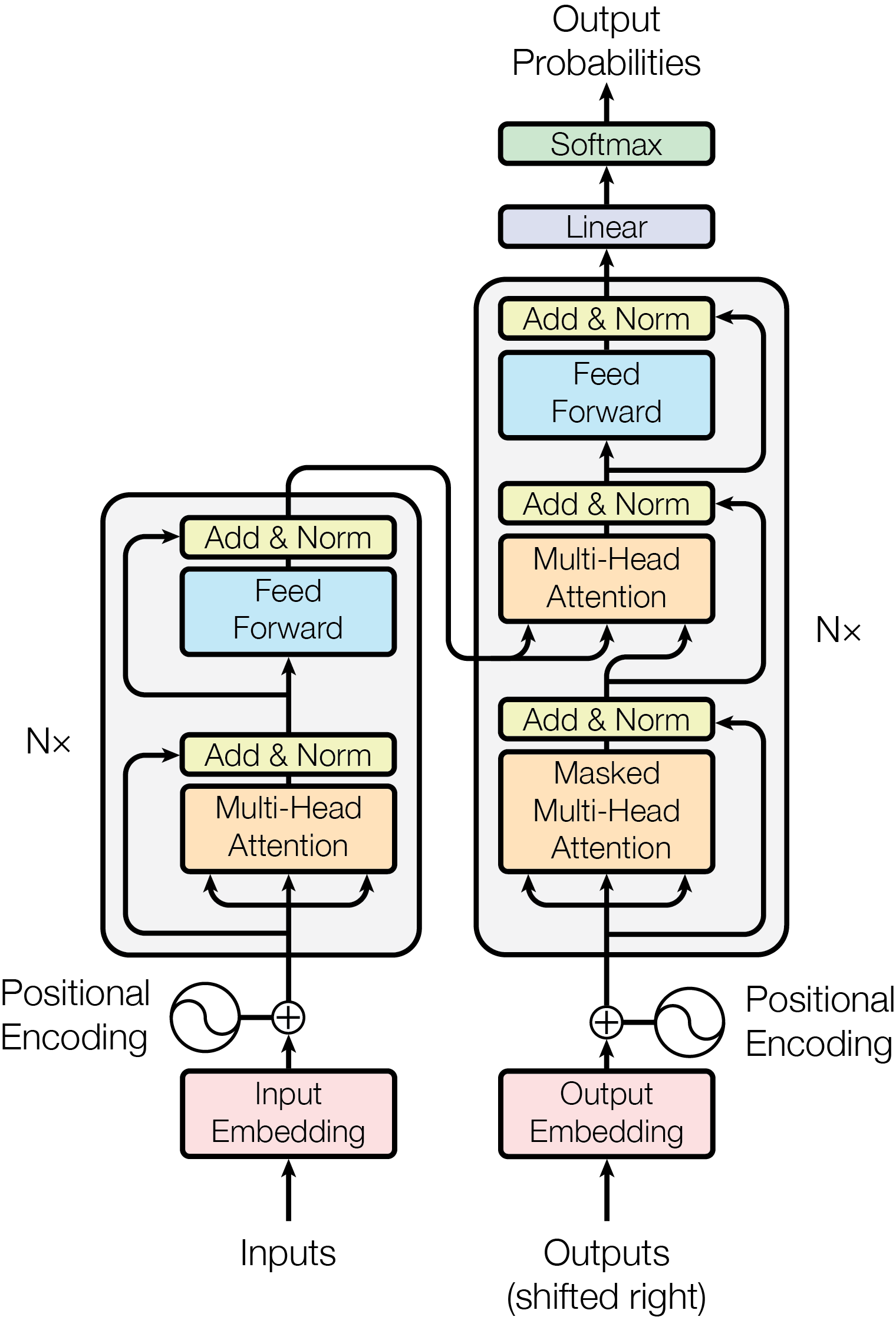
An encoder produces contextual representations of the source sequence; a decoder predicts the target sequence from earlier target tokens and those representations. Figure 1 shows the original architecture, including its residual connections and post-sublayer normalization.
3.1 Encoder and Decoder Stacks
Encoder:
The base encoder has six layers, each containing multi-head self-attention followed by a feed-forward network. Each sublayer has a residual connection followed by layer normalization. Embeddings and residual streams have dimension 512.
Decoder:
The six-layer decoder adds attention to the encoder output. Its own self-attention masks future positions, and shifted target embeddings prevent leakage of the token being predicted. This allows parallel training over known targets while preserving autoregressive generation.
3.2 Attention
A query compares with keys to determine weights, then returns a weighted sum of the corresponding values. Learned projections allow matching and retrieved content to occupy different vector spaces.
3.2.1 Scaled Dot-Product Attention
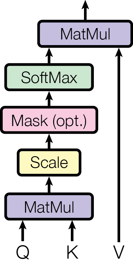
Scaled dot-product attention computes query–key dot products, divides by the square root of key dimension, applies softmax, and averages values. The scale controls growing score variance that could saturate softmax. Matrix multiplication makes this operation efficient for many queries at once.
Equation 1
| (1) |
3.2.2 Multi-Head Attention
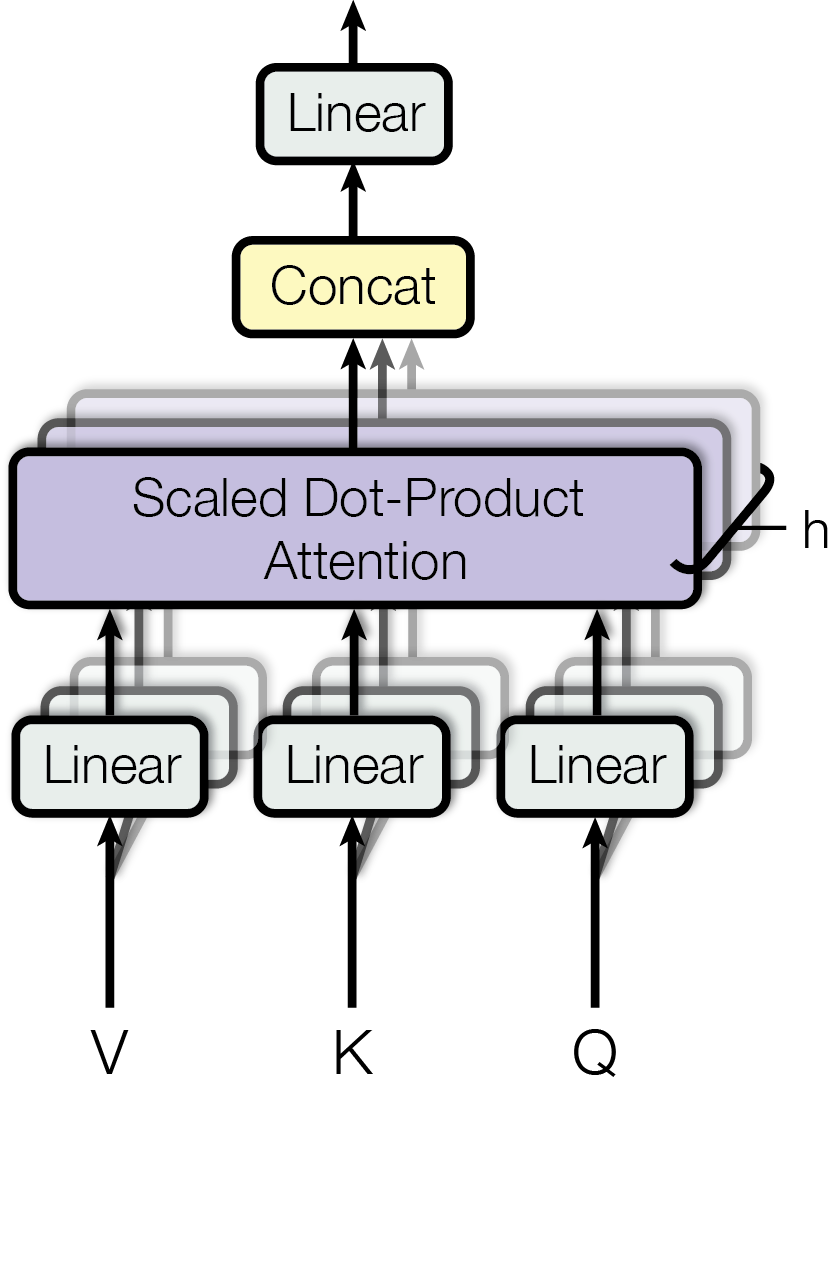
Each attention head independently projects queries, keys, and values; the outputs are concatenated and projected back. The base model uses eight heads with 64-dimensional keys and values. Multiple heads can retrieve different relationships without increasing cost to that of eight full-width attention operations.
Scaled Dot-Product Attention
Multi-Head Attention
Equation
3.2.3 Applications of Attention in our Model
Encoder self-attention connects all source positions. Decoder self-attention connects only the current and earlier target positions. Cross-attention uses decoder queries with encoder keys and values, giving each target position access to the source.
3.3 Position-wise Feed-Forward Networks
Every position receives the same two-layer feed-forward transformation within a layer: a linear map, ReLU, then another linear map. The base model expands dimension 512 to 2,048 and back. Different layers have different parameters.
Equation 2
| (2) |
3.4 Embeddings and Softmax
Learned embeddings represent input and output tokens. The paper shares weights between embedding matrices and the output softmax transformation, and scales embedding activations by the square root of model dimension.
3.5 Positional Encoding
Without recurrence, attention needs an explicit indication of position. Sines and cosines at multiple frequencies are added to token embeddings; learned positional embeddings perform similarly in the reported ablation. Extrapolation to longer sequences is a motivation for the sinusoidal choice, not a result demonstrated here.
Equation
4 Why Self-Attention
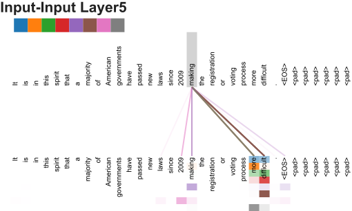
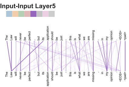
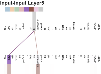
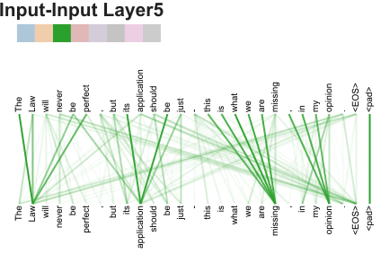
Self-attention offers constant-length connections and parallel operations across positions, but its full pairwise interaction cost grows quadratically with sequence length. Table 1 contrasts this with recurrence and convolutions. The appendix illustrates attention patterns related to syntax; such pictures suggest structure but do not by themselves establish a complete causal explanation of model behavior.
| Layer Type | Complexity per Layer | Sequential | Maximum Path Length |
|---|---|---|---|
| Operations | |||
| Self-Attention | |||
| Recurrent | |||
| Convolutional | |||
| Self-Attention (restricted) |
5 Training
5.1 Training Data and Batching
Training uses approximately 4.5 million English–German sentence pairs with a shared 37,000-token byte-pair vocabulary, and 36 million English–French pairs with 32,000 wordpieces. Batches group similar lengths and contain about 25,000 source and target tokens each.
5.2 Hardware and Schedule
Eight P100 GPUs train the base model for 100,000 steps, about twelve hours. The larger model uses 300,000 steps, about three and a half days. These are the paper’s hardware and workload measurements, not hardware-independent runtimes.
5.3 Optimizer
Adam uses a learning rate that first rises linearly for 4,000 warmup steps and then declines with the inverse square root of step count. The retained equation also accounts for model dimension.
Equation 3
| (3) |
5.4 Regularization
Regularization combines dropout and label smoothing, with the exact placements described below.
Residual Dropout
Dropout acts on sublayer outputs before residual addition and normalization, and on summed token and positional embeddings. The base rate is 0.1.
Label Smoothing
Label smoothing assigns some target probability away from the observed token. A value of 0.1 improves accuracy and BLEU while worsening perplexity, illustrating that these metrics need not move together.
6 Results
6.1 Machine Translation
The large model reaches 28.4 English–German BLEU; Table 2 and the abstract report 41.8 English–French BLEU, while the section’s prose says 41.0. This source inconsistency is retained rather than resolved by guessing. Results use checkpoint averaging, beam width four, and a length penalty. Training-cost estimates compare reported systems and should be interpreted with their hardware and methodological differences.
| Model | BLEU | Training Cost (FLOPs) | |||
|---|---|---|---|---|---|
| EN-DE | EN-FR | EN-DE | EN-FR | ||
| ByteNet[18] | 23.75 | ||||
| Deep-Att + PosUnk[39] | 39.2 | ||||
| GNMT + RL[38] | 24.6 | 39.92 | |||
| ConvS2S[9] | 25.16 | 40.46 | |||
| MoE[32] | 26.03 | 40.56 | |||
| Deep-Att + PosUnk Ensemble[39] | 40.4 | ||||
| GNMT + RL Ensemble[38] | 26.30 | 41.16 | |||
| ConvS2S Ensemble[9] | 26.36 | 41.29 | |||
| Transformer (base model) | 27.3 | 38.1 | |||
| Transformer (big) | 28.4 | 41.8 | |||
6.2 Model Variations
The translation development-set ablations favor multiple heads over a single head, sufficiently large key representations, larger models, and dropout. Learned and sinusoidal position embeddings are nearly tied. The table reports wordpiece perplexity, which should not be compared directly with word-level perplexity.
| train | PPL | BLEU | params | |||||||||
| steps | (dev) | (dev) | ||||||||||
| base | 6 | 512 | 2048 | 8 | 64 | 64 | 0.1 | 0.1 | 100K | 4.92 | 25.8 | 65 |
| (A) | 1 | 512 | 512 | 5.29 | 24.9 | |||||||
| 4 | 128 | 128 | 5.00 | 25.5 | ||||||||
| 16 | 32 | 32 | 4.91 | 25.8 | ||||||||
| 32 | 16 | 16 | 5.01 | 25.4 | ||||||||
| (B) | 16 | 5.16 | 25.1 | 58 | ||||||||
| 32 | 5.01 | 25.4 | 60 | |||||||||
| (C) | 2 | 6.11 | 23.7 | 36 | ||||||||
| 4 | 5.19 | 25.3 | 50 | |||||||||
| 8 | 4.88 | 25.5 | 80 | |||||||||
| 256 | 32 | 32 | 5.75 | 24.5 | 28 | |||||||
| 1024 | 128 | 128 | 4.66 | 26.0 | 168 | |||||||
| 1024 | 5.12 | 25.4 | 53 | |||||||||
| 4096 | 4.75 | 26.2 | 90 | |||||||||
| (D) | 0.0 | 5.77 | 24.6 | |||||||||
| 0.2 | 4.95 | 25.5 | ||||||||||
| 0.0 | 4.67 | 25.3 | ||||||||||
| 0.2 | 5.47 | 25.7 | ||||||||||
| (E) | positional embedding instead of sinusoids | 4.92 | 25.7 | |||||||||
| big | 6 | 1024 | 4096 | 16 | 0.3 | 300K | 4.33 | 26.4 | 213 | |||
6.3 English Constituency Parsing
A four-layer Transformer predicts linearized constituency trees. It reaches 91.3 F1 with the Wall Street Journal training set and 92.7 with additional semi-supervised data. The results show transfer beyond translation but do not surpass every listed parsing system; data regimes also differ across comparisons.
| Parser | Training | WSJ 23 F1 |
| Vinyals & Kaiser el al. (2014)[37] | WSJ only, discriminative | 88.3 |
| Petrov et al. (2006)[29] | WSJ only, discriminative | 90.4 |
| Zhu et al. (2013)[40] | WSJ only, discriminative | 90.4 |
| Dyer et al. (2016)[8] | WSJ only, discriminative | 91.7 |
| Transformer (4 layers) | WSJ only, discriminative | 91.3 |
| Zhu et al. (2013)[40] | semi-supervised | 91.3 |
| Huang & Harper (2009)[14] | semi-supervised | 91.3 |
| McClosky et al. (2006)[26] | semi-supervised | 92.1 |
| Vinyals & Kaiser el al. (2014)[37] | semi-supervised | 92.1 |
| Transformer (4 layers) | semi-supervised | 92.7 |
| Luong et al. (2015)[23] | multi-task | 93.0 |
| Dyer et al. (2016)[8] | generative | 93.3 |
7 Conclusion
Attention-only sequence transduction enables faster parallel training and strong translation results in this study. Suggested future work includes other modalities, restricted attention for long sequences, and less sequential generation. The authors release the Tensor2Tensor implementation.
Acknowledgements
The authors thank Nal Kalchbrenner and Stephan Gouws for comments and inspiration.
Attention Visualizations
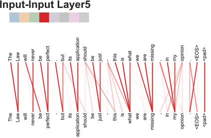
The retained attention maps show selected heads attending to long-distance verb dependencies, pronouns, and sentence structure. These examples illustrate specialization within one layer; they are qualitative examples rather than a systematic evaluation of interpretability.