At a glance
What information helps a convolutional pedestrian detector beyond the image itself? Controlled experiments compare semantic segmentation, edges, optical flow, disparity, and hand-crafted channels. Semantic context is most useful for small pedestrians; detailed boundaries help localization when images are enlarged.
HyperLearner then uses auxiliary feature maps as training supervision rather than extra inference inputs. A shared representation learns feature prediction and pedestrian detection jointly. Results improve over the tested baselines on KITTI, Cityscapes, and Caltech, with gains depending on image scale, task labels, and evaluation settings. The claims concern these 2017 systems and benchmarks, not current detector rankings.
1 Introduction
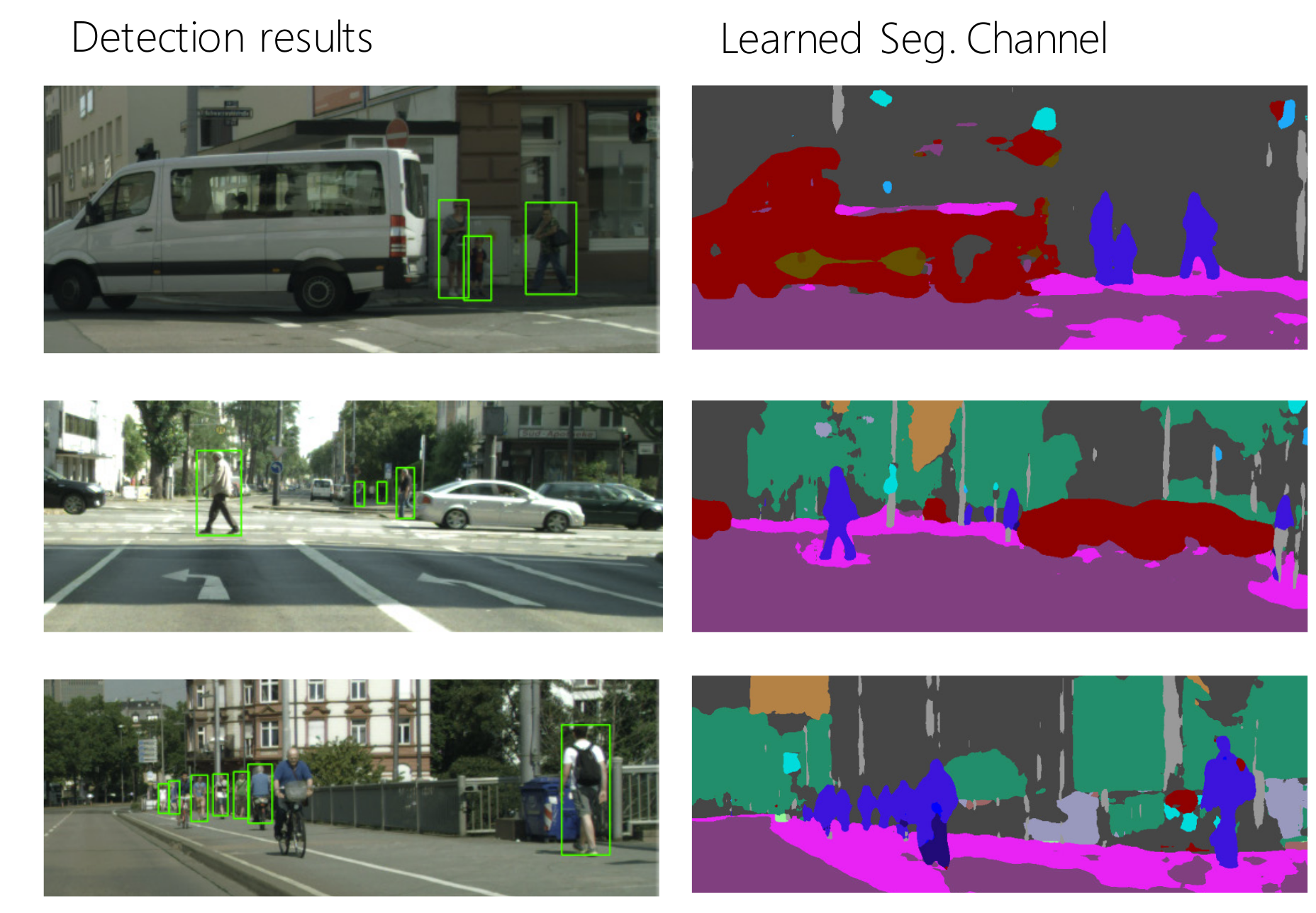
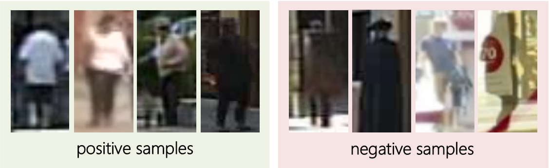
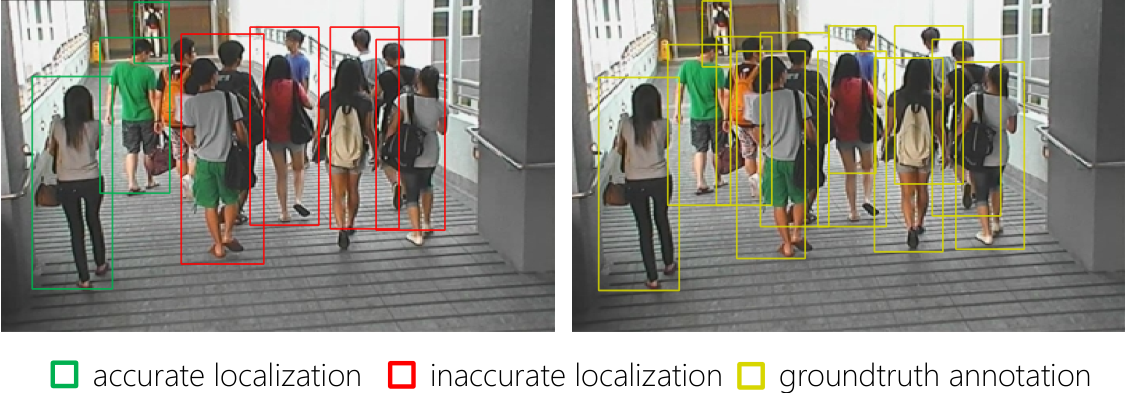
Small pedestrians can resemble signs, posts, and other background structures, making context valuable. Crowded scenes create a second problem: convolution and pooling blur boundaries between nearby people, so a detector may classify the scene correctly while placing boxes badly. Figure 1 illustrates both cases.
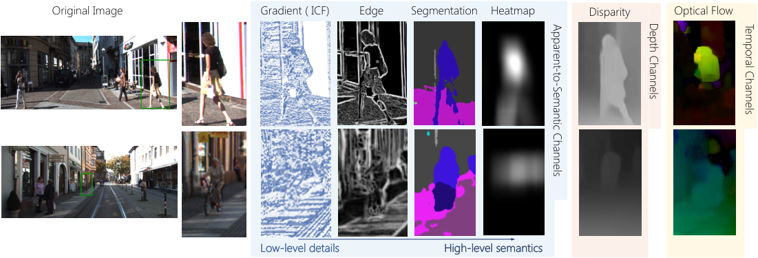
The study first supplies different channel features directly to a detector to isolate their value. It then trains a shared network to predict useful channels alongside detection, avoiding a separate feature-producing network or extra sensory input at deployment. Figure 2 distinguishes appearance, semantic, temporal, and depth cues.
2 Related work
Channel features had already helped boosted-forest pedestrian detectors, including gradient, optical-flow, and semantic representations. CNN detectors instead learn their own features and often use region proposals. This paper tests whether the earlier extra-channel advantage persists in a CNN pipeline, then connects feature aggregation with auxiliary-task supervision. [10] [23] [24] [33]
3 Channel features for pedestrian detection
The first experiments feed additional channels into a detector to compare the information they contribute.
3.1 Preliminaries
KITTI supplies pedestrian labels, adjacent video frames, and stereo images, enabling all three groups of cues to be tested. The authors use an established split of its 7,481 labeled images for training and validation. Easy, moderate, and hard settings differ in object scale and visibility; moderate is the principal metric. [26]
The baseline is Faster R-CNN with an ImageNet-pretrained VGG-16 backbone. Removing the conv5 layers preserves spatial resolution, and five anchor scales with seven aspect ratios target small objects. These modifications distinguish the baseline from the separately listed reproduction of standard Faster R-CNN. [24]
3.2 Introduction to channel features
Appearance-to-semantic cues include hand-crafted integral channels, learned HED edges, semantic segmentation, and a blurred segmentation heatmap. Their comparison separates fine boundaries from category context: blurring keeps semantics while removing localization detail. Segmentation is learned from MS-COCO; same-class neighboring people need not have distinct boundaries in that representation. [18] [31]
Optical flow represents temporal information from adjacent frames. DispNet estimates disparity from stereo images as the depth channel. These are auxiliary inputs in the initial analysis, unlike the later HyperLearner's training-only supervision. [21]
3.3 Integration techniques
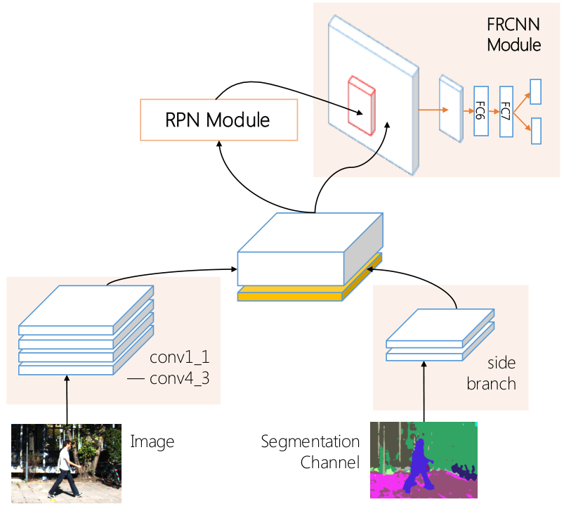
A shallow side branch converts each extra channel into a 128-channel map at one-eighth input resolution, concatenated with conv4_3 before proposal generation and detection. Two randomly initialized convolution layers work better than one layer or an independently pretrained side branch in the tested configurations. The authors hypothesize that pretraining makes the detector rely too heavily on the side branch; this is an interpretation of observed activations, not a general theorem. Table 1 retains the exact comparison.
| Model | Pedestrian | ||||
|---|---|---|---|---|---|
| #Convs | Init. W. | Mod | Easy | Hard | |
| O | N/A | N/A | 68.96 | 73.33 | 60.43 |
| A | 2 | random | 70.80 | 78.15 | 62.16 |
| B | 1 | random | 70.40 | 75.17 | 61.92 |
| C | 2 | pretrained | 69.92 | 77.33 | 61.65 |
| Model | Recall | |||
|---|---|---|---|---|
| all scales | ||||
| Baseline | 21.3% | 87.6% | 96.8% | 70.0% |
| +Segmentation | 35.6% | 88.2% | 96.8% | 74.0% |
3.4 Comparison and analysis
At original image scale, segmentation and blurred heatmaps give the largest gains; extra raw-image input gives little consistent improvement. At 70% precision, segmentation raises overall recall from 70.0% to 74.0%, with the largest increase for pedestrians up to 80 pixels tall: 21.3% to 35.6%. This supports a role for semantic context in small-object discrimination.
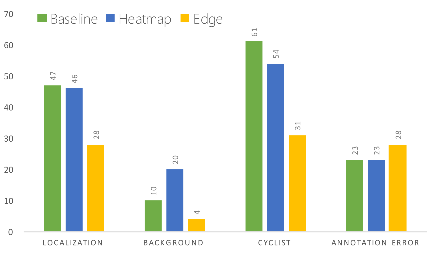
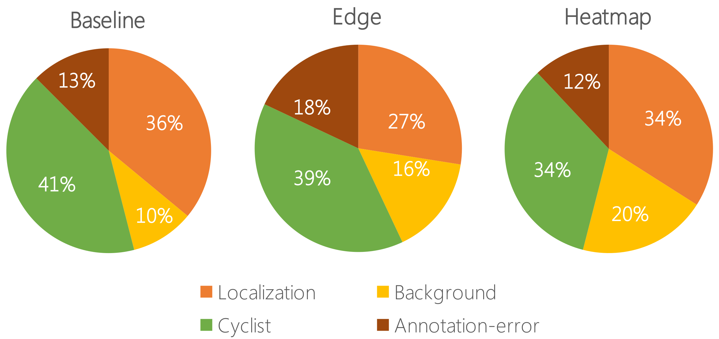
At double scale, edge and segmentation cues remain useful while the boundary-free heatmap contributes less. An error analysis on about 800 validation images and the top 200 false positives links edges to improved localization. The reported 9-point localization-error reduction is relative to the baseline's error composition, not an overall detection-accuracy gain. Optical flow mainly helps at original scale; disparity behaves more like semantic context than a uniformly useful depth measurement. All values and difficulty-specific differences remain in Tables 2–3 and Figure 4.
| Model | Pedestrian 1x Input | Improvement | Pedestrian 2x Input | Improvement | ||||||||||
|---|---|---|---|---|---|---|---|---|---|---|---|---|---|---|
| Mod | Easy | Hard | Mod | Easy | Hard | Avg | Mod | Easy | Hard | Mod | Easy | Hard | Avg | |
| Fr-RCNN* [24] | 59.29 | 64.53 | 53.01 | - | - | - | - | 71.05 | 76.00 | 62.08 | - | - | - | - |
| MS-CNN [2] | 68.37 | 73.70 | 60.72 | - | - | - | - | 72.26 | 76.38 | 64.08 | - | - | - | - |
| Our Baseline | 68.96 | 73.33 | 60.43 | - | - | - | - | 71.21 | 77.73 | 62.19 | - | - | - | - |
| + Original img | 68.63 | 76.61 | 60.45 | -0.33 | +3.28 | +0.02 | +0.99 | 71.33 | 76.72 | 62.17 | +0.12 | -1.01 | -0.02 | -0.30 |
| + ICF | 68.40 | 73.56 | 60.20 | -0.56 | +0.23 | -0.23 | -0.19 | 71.80 | 77.40 | 62.79 | +0.59 | -0.33 | +0.60 | +0.29 |
| + Edge | 69.49 | 76.28 | 60.89 | +0.53 | +2.95 | +0.46 | +1.31 | 72.34 | 78.32 | 63.28 | +1.13 | +0.59 | +1.09 | +0.94 |
| + Segmentation | 70.80 | 78.15 | 62.16 | +1.84 | +4.82 | +1.73 | +2.80 | 72.54 | 78.49 | 63.61 | +1.33 | +0.76 | +1.42 | +1.17 |
| + Heatmap | 70.33 | 78.03 | 61.75 | +1.37 | +4.70 | +1.32 | +2.46 | 71.39 | 77.64 | 62.34 | +0.18 | -0.09 | +0.15 | +0.08 |
| + Disparity | 70.03 | 77.74 | 61.48 | +1.07 | +4.41 | +1.05 | +2.18 | 71.72 | 77.52 | 62.47 | +0.51 | -0.21 | +0.28 | +0.19 |
| + Optical Flow | 69.39 | 77.07 | 60.79 | +0.43 | +3.74 | +0.36 | +1.51 | 71.13 | 76.85 | 62.24 | -0.08 | -0.88 | +0.05 | -0.25 |
4 Jointly learn the channel features
Computing auxiliary maps at inference can be expensive. HyperLearner instead learns to predict the useful maps as an auxiliary task, allowing their supervision to shape the features used by the detector.
4.1 HyperLearner
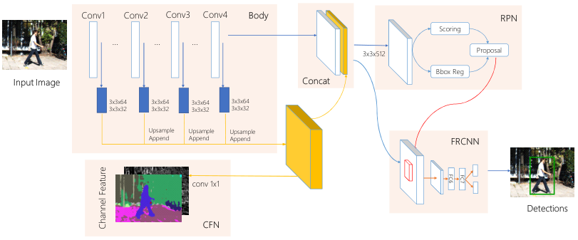
HyperLearner has a shared body, a channel-feature network, a region-proposal network, and a Fast R-CNN head. Features from VGG layers conv1_2, conv2_2, conv3_3, and conv4_3 each pass through two convolutions to produce 32 channels. Upsampling and concatenation create a common-resolution aggregated map.
The channel-feature network predicts the auxiliary map from that representation. Proposal generation and detection use both the aggregated map and conv4_3, so auxiliary supervision changes their shared features. At inference, only the original image is required; the external network that produced training targets is unnecessary. Figure 5 preserves the full architecture.
4.2 Training Details
Training combines pixel-level feature prediction with the usual proposal and detection classification/regression losses. Binary edge maps use class-balanced cross-entropy; multiclass segmentation uses cross-entropy, and other auxiliary tasks use mean-squared error. The target map is S, the predicted map C, and the pixel loss is averaged over its H by W locations. Positive pixels have targets above 0.5: their weight is one minus the positive fraction, while negative pixels receive the positive fraction. All four detector-loss weights are one.
Training proceeds in four stages: train the channel-feature network with pretrained body layers fixed; train the proposal network with the body and auxiliary network fixed; train the detection head while fixing earlier components; then optimize all layers jointly. Proposal coordinates are treated as fixed when differentiating the detection-head loss.
Equations
5 Experiments and results
KITTI, Cityscapes, and Caltech test the approach under different image scales and supervision. A HyperNet control keeps the multilevel aggregation but removes auxiliary feature supervision, separating the effect of architecture from the effect of the extra training task.
5.1 KITTI Dataset
At original scale, KITTI moderate performance rises from 69.80 for the baseline to 71.15 with segmentation supervision and 71.25 with edge supervision; aggregation alone reaches 69.72. At double scale, the corresponding baseline and edge-supervised results are 71.73 and 72.51, with HyperNet at 72.23. Gains are therefore larger at original resolution, and architecture alone explains some high-resolution improvement.
Results differ across easy, moderate, and hard settings: Table 4 does not show that either auxiliary task uniformly wins every metric. These are validation-set comparisons with the stated modified detector, not results on KITTI's held-out official test set.
| Model | 1x input | 2x input | ||||
|---|---|---|---|---|---|---|
| Mod | Easy | Hard | Mod | Easy | Hard | |
| Fr-RCNN* [24] | 59.29 | 64.53 | 53.01 | 71.05 | 76.00 | 62.08 |
| MS-CNN [2] | 68.37 | 73.70 | 60.72 | 72.26 | 76.38 | 64.08 |
| Baseline | 69.80 | 74.37 | 61.20 | 71.73 | 77.84 | 62.30 |
| HyperNet | 69.72 | 76.91 | 61.10 | 72.23 | 77.96 | 63.43 |
| +Segmentation | 71.15 | 79.43 | 62.34 | 72.35 | 79.17 | 62.34 |
| +Edge | 71.25 | 78.43 | 62.15 | 72.51 | 78.51 | 63.24 |
*: Fr-RCNN follows setting as [24] while baseline model is Faster-RCNN with slightly different parameters. See also Table 3.
5.2 Cityscapes dataset
Cityscapes supplies human segmentation labels directly, so the auxiliary task uses person pixels rather than predictions from a separately trained segmentation model. Experiments use the finely annotated training and validation images.
At 540p, average precision increases from 74.97 to 77.22 while measured per-image latency rises from 130 to 140 ms on one Titan X GPU. At 720p, precision rises from 86.89 to 87.67 and latency from 240 to 250 ms. The detection evaluation derives boxes from person polygons and excludes small, heavily occluded, cyclist, and person-group cases as detailed in Table 5. These restrictions bound the result's scope.
5.3 Caltech dataset
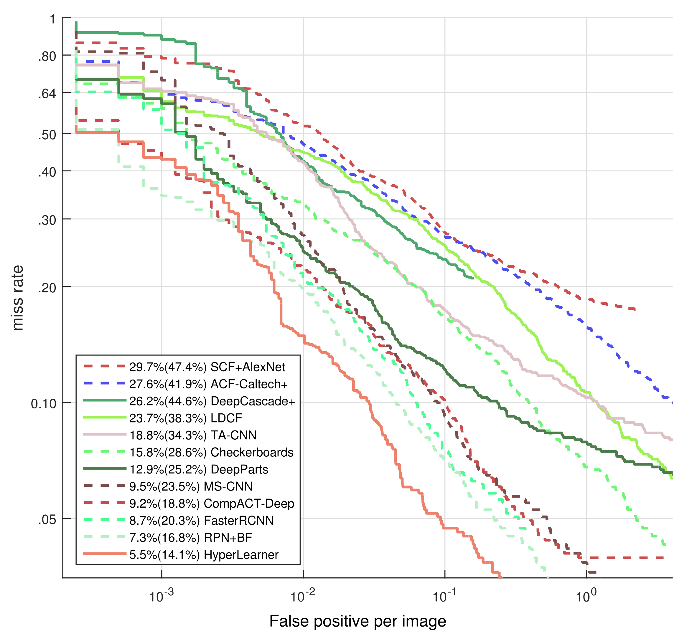
Caltech evaluation uses the refined annotations for both training and testing and evaluates 4,024 test frames. Figure 7 compares miss-rate curves on the reasonable subset using the updated labels. The authors report the strongest results among the methods in that historical comparison; the curve and protocol should accompany the ranking claim. [11] [34]
6 Summary
The experiments support two complementary roles for auxiliary information: semantic context helps disambiguate small pedestrians, while boundaries help localize people in higher-resolution images. HyperLearner transfers those cues through a shared representation during training, avoiding extra inference inputs.
The evidence comes from specific backbones, tasks, scales, labels, and benchmark subsets. Auxiliary supervision and multilevel aggregation both matter, and the tables show nonuniform gains. Generalization to other detector families or unrestricted crowded-scene deployment is not established by these experiments.
| Model | 540p input | 720p input | Improvement | |||
|---|---|---|---|---|---|---|
| Speed | AP | Speed | AP | 540p | 720p | |
| Baseline | 130ms | 74.97 | 240ms | 86.89 | - | - |
| HyperNet | 140ms | 74.30 | 250ms | 86.67 | -0.53 | -0.22 |
| Jointsegmap | 140ms | 77.22 | 250ms | 87.67 | +2.25 | +0.78 |