At a glance
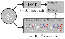
Message Passing Neural Networks unify several graph architectures through learned messages, node updates, and a permutation-invariant readout. On QM9, an edge-conditioned message function with set2set readout reaches chemical-accuracy thresholds for 11 of 13 properties. These thresholds are measured against approximate computational labels, not precise experimental chemistry.
1 Introduction
Molecular prediction should respect invariance to atom ordering while learning useful features from bonds and geometry. QM9 provides a controlled test with small molecules and density-functional-theory targets. The strongest model improves every compared target, while the tower variant lowers computation. The paper argues for careful application-driven comparisons within a shared framework.
2 Message Passing Neural Networks
During each message-passing step, a node aggregates messages from its neighbors and updates its hidden state. A readout then pools node states into a graph prediction and must ignore node order. Existing fingerprint networks, gated graph networks, interaction networks, molecular convolutions, tensor networks, and spectral methods differ in these component functions. Edge states can also evolve. The preserved formulas show the exact correspondences.
Equations 1–4
| (1) | ||||
| (2) |
| (3) |
| (4) |
2.1 Moving Forward
The proposed framework organizes existing models rather than claiming that message passing itself is new. Useful progress requires strong empirical studies and scalable implementations; computational cost remains a limitation.
3 Related Work
Quantum calculations trade accuracy against cost, and density functional theory has both systematic and random error. Earlier machine-learning surrogates often used engineered descriptors, sometimes requiring augmentation to approximate permutation invariance. Learned graph representations offer a more direct structural bias, but predicting a simulator still inherits its target limitations.
4 QM9 Dataset
QM9 contains small organic molecules built from hydrogen, carbon, oxygen, nitrogen, and fluorine, with at most nine heavy atoms. The 13 targets cover atomization thermodynamics, vibrational properties, orbital energies, charge distribution, and polarizability. Models are evaluated both with computed geometry and with graph topology alone; those are different information settings.
5 MPNN Variants
Variants start from gated graph networks with shared weights across propagation steps and GRU updates. Atom features initialize node states. Undirected molecular bonds are represented as paired directed channels, permitting separate incoming and outgoing message parameters.
5.1 Message Functions
The baseline chooses a message matrix from a discrete edge type. The edge network instead generates that matrix from a continuous edge-feature vector, allowing raw interatomic distance. A pair-message network also sees the receiving node’s state, but proves harder to train and performs worse in the reported comparisons.
5.2 Virtual Graph Elements
Virtual edges connect otherwise unrelated atom pairs; a master node creates global scratch space connected to every atom. Both reduce the number of propagation steps needed for distant atoms to interact, at an additional computational cost.
5.3 Readout Functions
The readout is either the gated graph network’s weighted sum or a set2set module that repeatedly attends over node representations. The latter produces a richer order-invariant graph embedding before the final prediction network.
5.4 Multiple Towers
Towers split each node state into smaller independent message-passing channels, then mix their outputs at each node. For dense graphs, the main message cost drops by a factor equal to the tower count, excluding mixing overhead. Eight towers give about a twofold measured inference speedup in the illustrated configuration.
Equation 5
| (5) |
6 Input Representation
Inputs include atom identity and chemical features, discrete bond type, and optionally distance. Spatial information enters as hand-chosen distance bins or raw distances. Treating hydrogen as explicit graph nodes helps accuracy on several targets but increases training cost by roughly tenfold in these experiments.
| Feature | Description | |
|---|---|---|
| Atom type | H, C, N, O, F (one-hot) | |
| Atomic number | Number of protons (integer) | |
| Acceptor | Accepts electrons (binary) | |
| Donor | Donates electrons (binary) | |
| Aromatic | In an aromatic system (binary) | |
| Hybridization | sp, sp2, sp3 (one-hot or null) | |
| Number of Hydrogens | (integer) |
7 Training
The 130,462 usable molecules are split into 10,000 validation, 10,000 test, and the remainder for training. Models use Adam, batch size 20, standardized targets, and squared-error training, while evaluation reports absolute error. Random hyperparameter searches and validation-based early stopping select models. Most main comparisons train one network per target.
8 Results
The best individual-target model combines edge-network messages, explicit hydrogen, and set2set readout; a five-model ensemble improves further. Geometry substantially helps. Long-range communication also improves graph-only models. A crucial caveat: some graph-only and tower ablations use partial charges computed by the target simulator, which would be unavailable in an applied setting. The headline state-of-the-art results exclude that feature. Jointly predicting all targets generally underperforms individual training.
| Target | BAML | BOB | CM | ECFP4 | HDAD | GC | GG-NN | DTNN | enn-s2s | enn-s2s-ens5 |
|---|---|---|---|---|---|---|---|---|---|---|
| mu | 4.34 | 4.23 | 4.49 | 4.82 | 3.34 | 0.70 | 1.22 | - | 0.30 | 0.20 |
| alpha | 3.01 | 2.98 | 4.33 | 34.54 | 1.75 | 2.27 | 1.55 | - | 0.92 | 0.68 |
| HOMO | 2.20 | 2.20 | 3.09 | 2.89 | 1.54 | 1.18 | 1.17 | - | 0.99 | 0.74 |
| LUMO | 2.76 | 2.74 | 4.26 | 3.10 | 1.96 | 1.10 | 1.08 | - | 0.87 | 0.65 |
| gap | 3.28 | 3.41 | 5.32 | 3.86 | 2.49 | 1.78 | 1.70 | - | 1.60 | 1.23 |
| R2 | 3.25 | 0.80 | 2.83 | 90.68 | 1.35 | 4.73 | 3.99 | - | 0.15 | 0.14 |
| ZPVE | 3.31 | 3.40 | 4.80 | 241.58 | 1.91 | 9.75 | 2.52 | - | 1.27 | 1.10 |
| U0 | 1.21 | 1.43 | 2.98 | 85.01 | 0.58 | 3.02 | 0.83 | - | 0.45 | 0.33 |
| U | 1.22 | 1.44 | 2.99 | 85.59 | 0.59 | 3.16 | 0.86 | - | 0.45 | 0.34 |
| H | 1.22 | 1.44 | 2.99 | 86.21 | 0.59 | 3.19 | 0.81 | - | 0.39 | 0.30 |
| G | 1.20 | 1.42 | 2.97 | 78.36 | 0.59 | 2.95 | 0.78 | .8422 2 As reported in Schütt et al. (2017). The model was trained on a different train/test split with 100k training samples vs 110k used in our experiments. | 0.44 | 0.34 |
| Cv | 1.64 | 1.83 | 2.36 | 30.29 | 0.88 | 1.45 | 1.19 | - | 0.80 | 0.62 |
| Omega | 0.27 | 0.35 | 1.32 | 1.47 | 0.34 | 0.32 | 0.53 | - | 0.19 | 0.15 |
| Average | 2.17 | 2.08 | 3.37 | 53.97 | 1.35 | 2.59 | 1.36 | - | 0.68 | 0.52 |
9 Conclusions and Future Work
Learned graph representations are competitive surrogates for small-molecule calculations, but the study does not establish transfer to larger molecules or experimental ground truth. Fully connected distance graphs change message counts and distance distributions with molecule size. Larger and more accurate benchmarks, scalable interactions, and attention over messages are proposed next steps.
Acknowledgements
The authors acknowledge discussions with colleagues and Adrian Roitberg’s identification of the partial-charge input issue.
10 Appendix
10.1 Interpretation of Laplacian based models as MPNNs
Spectral graph convolutions can be rewritten as sums of transformed neighboring node states. Expanding the Laplacian-eigenvector operator exposes a matrix-valued message coefficient for each ordered node pair, followed by a pointwise update. The preserved derivation establishes its relation to the general framework.
Equations 6
| (6) |
10.1.1 The special case of Kipf and Welling (2016)
The first-order normalized graph-convolution rule adds self-loops, averages neighbor features with degree-based scalar weights, and applies a learned transform and nonlinearity. It is therefore a message-passing special case with a particularly simple message function.
Equations 7–8
| (7) |
| (8) |
10.2 A More Detailed Description of the Quantum Properties
Atomization energies describe molecular binding under specified thermodynamic conditions. Vibrational targets measure the highest fundamental frequency and zero-point energy. Orbital targets describe occupied/unoccupied levels and their gap. Spatial extent, dipole magnitude, and polarizability characterize electron distribution and response to an external field. Definitions should be read with the target units retained in the source tables.
10.3 Chemical Accuracy and DFT Error
Reported error ratios divide a model’s mean absolute error by a target-specific chemical-accuracy estimate. A ratio below one meets that threshold relative to the dataset labels. Multiplying by the tabulated threshold recovers absolute error; the separately tabulated density-functional-theory errors quantify a different approximation.
10.4 Additional Results
The appendix retains learning-size, input-feature, tower, and message-function comparisons for every target. Some targets remain strong with only 11,000 training examples. Long-range graph mechanisms and towers help several settings, while pair messages underperform edge networks. Search budgets differ across the tower comparisons, and one baseline comparison reports minimum test error across trials; these details limit a clean causal interpretation of the gains.
| Target | N=11k | N=35k | N=58k | N=82k | N=110k |
|---|---|---|---|---|---|
| mu | 1.28 | 0.55 | 0.44 | 0.32 | 0.30 |
| alpha | 2.76 | 1.59 | 1.26 | 1.09 | 0.92 |
| HOMO | 2.33 | 1.50 | 1.34 | 1.19 | 0.99 |
| LUMO | 2.18 | 1.47 | 1.19 | 1.10 | 0.87 |
| gap | 3.53 | 2.34 | 2.07 | 1.84 | 1.60 |
| R2 | 0.28 | 0.22 | 0.21 | 0.21 | 0.15 |
| ZPVE | 2.52 | 1.78 | 1.69 | 1.68 | 1.27 |
| U0 | 1.24 | 0.69 | 0.58 | 0.62 | 0.45 |
| U | 1.05 | 0.69 | 0.60 | 0.52 | 0.45 |
| H | 1.14 | 0.64 | 0.65 | 0.53 | 0.39 |
| G | 1.23 | 0.62 | 0.64 | 0.49 | 0.44 |
| Cv | 1.99 | 1.24 | 0.93 | 0.87 | 0.80 |
| Omega | 0.28 | 0.25 | 0.24 | 0.15 | 0.19 |
| Target | GG-NN | ve | mn | s2s |
|---|---|---|---|---|
| mu | 3.94 | 3.76 | 4.02 | 3.81 |
| alpha | 2.43 | 2.07 | 2.01 | 2.04 |
| HOMO | 1.80 | 1.60 | 1.67 | 1.71 |
| LUMO | 1.73 | 1.48 | 1.48 | 1.41 |
| gap | 2.48 | 2.33 | 2.23 | 2.26 |
| R2 | 14.74 | 17.11 | 13.16 | 13.67 |
| ZPVE | 5.93 | 3.21 | 3.26 | 3.02 |
| U0 | 1.98 | 0.89 | 0.90 | 0.72 |
| U | 2.48 | 0.93 | 0.99 | 0.79 |
| H | 2.19 | 0.86 | 0.95 | 0.80 |
| G | 2.13 | 0.85 | 1.02 | 0.74 |
| Cv | 1.96 | 1.61 | 1.63 | 1.71 |
| Omega | 1.28 | 1.05 | 0.78 | 0.78 |
| Average | 3.47 | 2.90 | 2.62 | 2.57 |
| Target | GG-NN-j | tow8-j | GG-NN-i | tow8-i |
|---|---|---|---|---|
| mu | 2.73 | 2.47 | 2.16 | 2.23 |
| alpha | 1.66 | 1.50 | 1.47 | 1.34 |
| HOMO | 1.33 | 1.19 | 1.27 | 1.20 |
| LUMO | 1.28 | 1.12 | 1.24 | 1.11 |
| gap | 1.73 | 1.55 | 1.78 | 1.68 |
| R2 | 6.07 | 6.16 | 4.78 | 4.11 |
| ZPVE | 4.07 | 3.43 | 2.70 | 2.54 |
| U0 | 1.00 | 0.86 | 0.71 | 0.55 |
| U | 1.01 | 0.88 | 0.65 | 0.52 |
| H | 1.01 | 0.88 | 0.68 | 0.50 |
| G | 0.99 | 0.85 | 0.66 | 0.50 |
| Cv | 1.40 | 1.27 | 1.27 | 1.09 |
| Omega | 0.66 | 0.62 | 0.57 | 0.50 |
| Average | 1.92 | 1.75 | 1.53 | 1.37 |
| Target | pm-j | enn-j |
|---|---|---|
| mu | 2.10 | 2.24 |
| alpha | 2.30 | 1.48 |
| HOMO | 1.20 | 1.30 |
| LUMO | 1.46 | 1.20 |
| gap | 1.80 | 1.75 |
| R2 | 10.87 | 2.41 |
| ZPVE | 16.53 | 3.85 |
| U0 | 3.16 | 0.92 |
| U | 3.18 | 0.93 |
| H | 3.20 | 0.93 |
| G | 2.97 | 0.92 |
| Cv | 2.17 | 1.28 |
| Omega | 0.83 | 0.74 |
| Average | 3.98 | 1.53 |
| Target | no distance | distance | dist + exp hydrogen |
|---|---|---|---|
| mu | 3.81 | 0.95 | 0.30 |
| alpha | 2.04 | 1.18 | 0.92 |
| HOMO | 1.71 | 1.10 | 0.99 |
| LUMO | 1.41 | 1.06 | 0.87 |
| gap | 2.26 | 1.74 | 1.60 |
| R2 | 13.67 | 0.57 | 0.15 |
| ZPVE | 3.02 | 2.57 | 1.27 |
| U0 | 0.72 | 0.55 | 0.45 |
| U | 0.79 | 0.55 | 0.45 |
| H | 0.80 | 0.59 | 0.39 |
| G | 0.74 | 0.55 | 0.44 |
| Cv | 1.71 | 0.99 | 0.80 |
| Omega | 0.78 | 0.41 | 0.19 |
| Average | 2.57 | 0.98 | 0.68 |