A small local change to one oscillator can stop a coordinated network of rhythmic movement primitives, then allow its rhythm to resume. Contraction theory supplies conditions for this sparse inhibition, for composing primitives, and for tolerating oscillator heterogeneity. MIT Cheetah experiments demonstrate start–stop transitions in an amble gait; the analysis certifies the primitive dynamics rather than full contact and body stability.
1 Introduction
Dynamic Movement Primitives (DMPs) represent reusable attractor dynamics. The paper analyzes their interconnections through contraction and transverse contraction, then introduces spatially sparse inhibition of rhythmic DMPs. Its central distinction is between convergence to a trajectory or equilibrium and convergence to a periodic orbit up to phase. [32], [21], [33].
2 Dynamic Movement Primitives
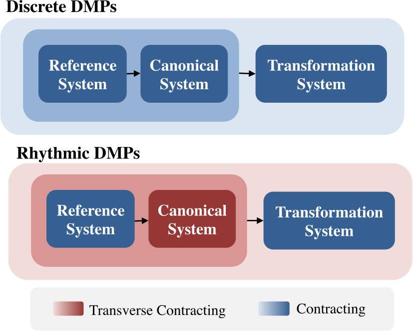
A DMP is treated as a hierarchy of three systems: a reference filter processes commands, a canonical system defines phase, and a transformation system produces the desired movement. This common structure supports a modular stability analysis across different implementations.
2.1 Discrete (Point-To-Point) Motion Primitives
A damped spring converges to a goal while a decaying phase variable controls a learned forcing function. Because the forcing fades, it can shape the transient without changing the terminal attractor. Reference filtering smooths changes to external goal commands.
Equations 1–4
(1)
(2)
(3)
(4)
2.2 Rhythmic Motion Primitives
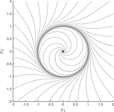
For rhythmic motion, an Andronov–Hopf oscillator replaces the decaying phase variable. Phase-dependent forcing shapes the output, while reference filters can smoothly adjust the oscillation center and amplitude. The canonical system retains a limit cycle rather than converging to a single point.
Equations 5–7
(5)
(6)
(7)
2.3 Commonalities
Reference and transformation subsystems are contracting in their own states. The canonical subsystem is contracting for discrete movements or transversely contracting for rhythmic movements. The combination results below propagate these properties through the hierarchy.
The analysis establishes stability certificates for individual primitives, transformed primitives, and coupled networks.
3.1 Contraction Preliminaries
Contraction means that trajectories converge exponentially in a uniformly positive-definite metric within a forward-invariant region. Transverse contraction requires convergence only perpendicular to the flow, allowing persistent phase differences. On a compact strictly forward-invariant region without equilibria, it implies convergence to a unique limit cycle. The metric and associated generalized Jacobian express these conditions.
Equations 11–16
(11)
(12)
(13)
(14)
(15)
(16)
3.2 Scaling in Space and Time
A smooth invertible spatial transformation transports the contraction metric through its inverse Jacobian. Positive time scaling likewise preserves the contraction structure under the stated uniform conditions. Rotation, translation, and scaling are special cases; more general diffeomorphisms can reshape the attractor while retaining the appropriate certificate.
Equation 17
(17)
3.3 Combination Properties
A hierarchy of contracting systems remains contracting. Combining one transversely contracting subsystem with a contracting upstream or downstream subsystem preserves transverse contraction under the stated assumptions. These results permit analyzing a DMP through its components.
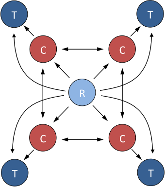
Discrete DMP hierarchies inherit contraction; rhythmic hierarchies inherit transverse contraction for a fixed external reference. In coupled rhythmic networks, connected diffusive coupling strong enough to dominate the individual Jacobians synchronizes canonical states and yields a common stable rhythm. The displayed spectral condition is sufficient, and alternative norms may reduce conservatism.
Figure 1: Contraction analysis readily admits stability specifications for discrete and rhythmic DMPs.Equations 18–20
(18)
(19)
(20)
Figure 2: Network of coupled rhythmic DMPs with common reference system (R), coupled canonical systems (C), and transformation systems (T).Equation 21
(21)
3.5 Coupled Oscillators with Multiple Frequencies
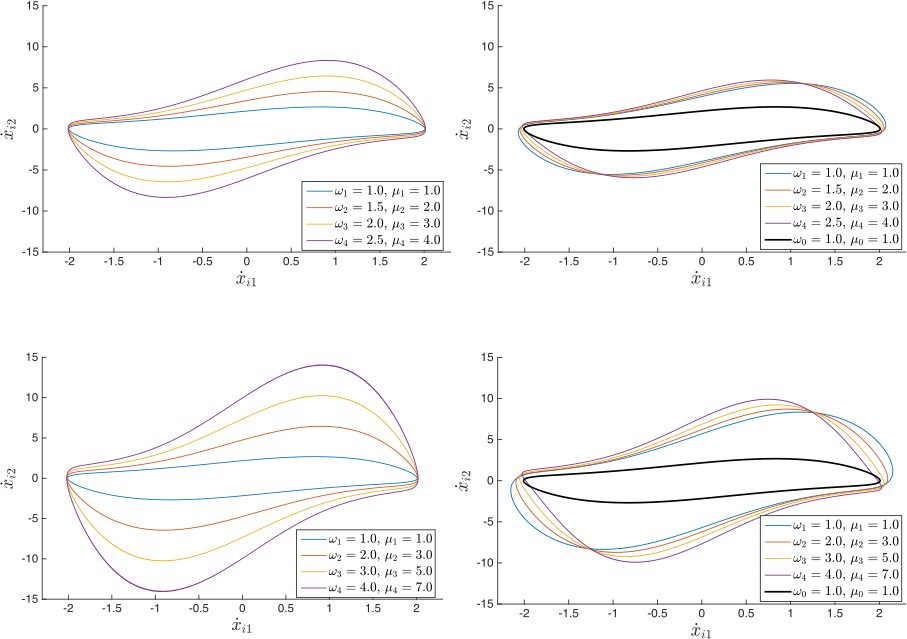
A transversely contracting network without equilibria remains so for sufficiently small continuous parameter changes. Thus nearby heterogeneous oscillators converge to a shared periodic orbit even when their natural frequencies differ. Parameter mismatch produces bounded synchronization and orbit deviations proportional to disturbance magnitude and inversely related to contraction rate; the result is local in parameter space, not unrestricted heterogeneity.
Equations 22–23
(22)
(23)
Figure 3: Left: Uncoupled heterogeneous Van der Pol oscillators with and . Right: With diffusive coupling . New results guarantee a common period for changes in parameter heterogeneity within an open set, and continuity of the resulting periodic orbit across parameters.
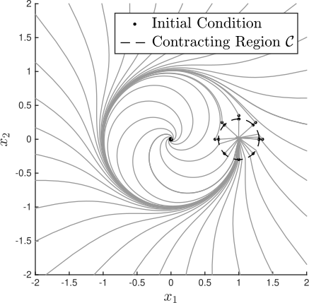
Sparse inhibition changes a rhythmic network into a contracting one by modifying only a small portion of its canonical dynamics.
4.1 Local Influence of Contracting Dynamics
When a transverse-contraction region overlaps a forward-invariant contraction region, trajectories in their union converge to the unique equilibrium in the overlap. A sufficiently strong contracting vector field can dominate another smooth field on a compact region. These facts enable local capture of an orbit and motivate sequential composition.
Equations
4.2 Application to Sparse Inhibition of Rhythmic DMPs
Diffusive coupling plus a contracting influence at one node creates a contracting network contribution. If coupling and inhibition are strong enough, that contribution suppresses the entire network’s rhythm. Inhibition can activate when the controlled oscillator enters a selected region. A directed-network extension requires every node to be reachable from the inhibited node.
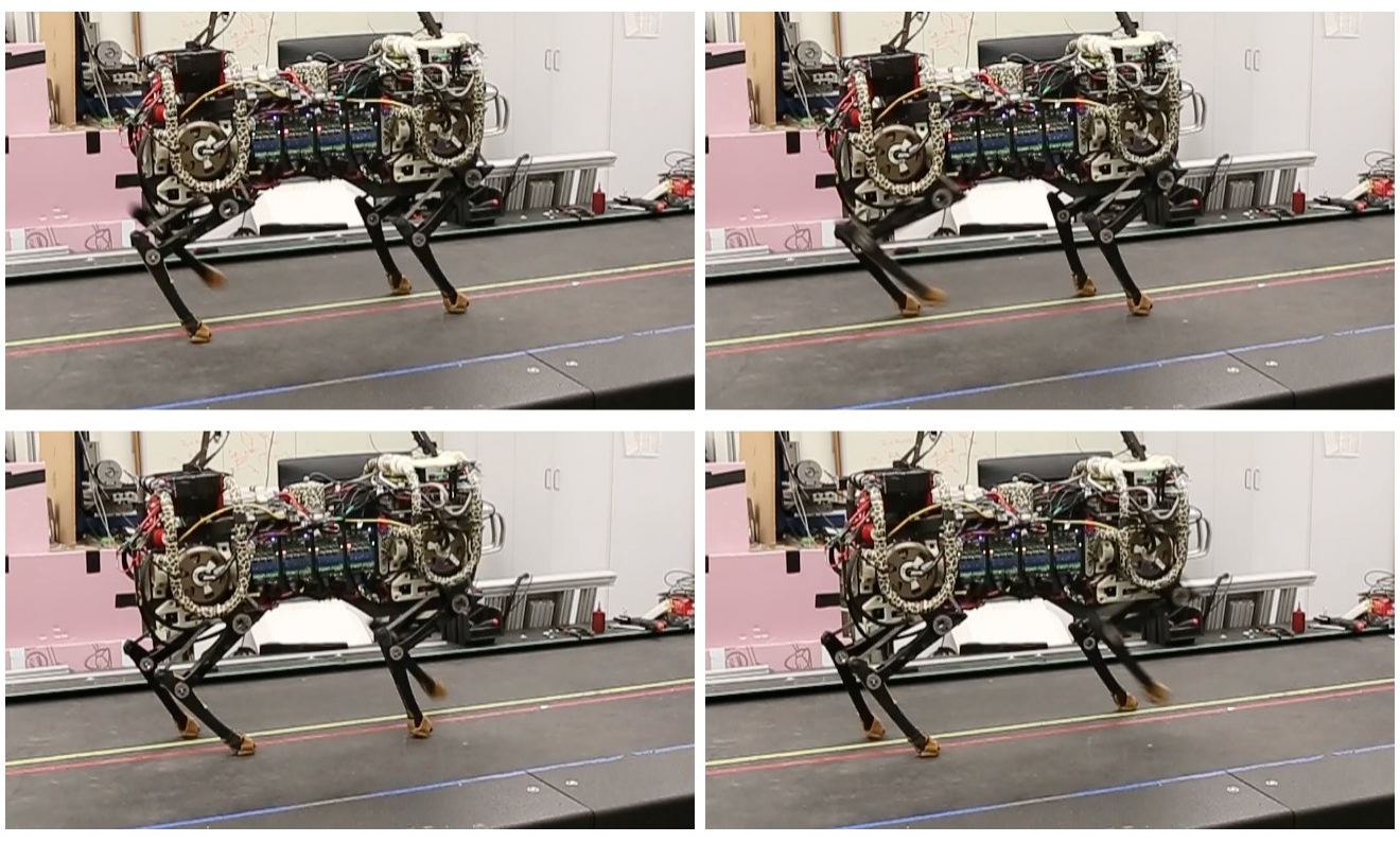
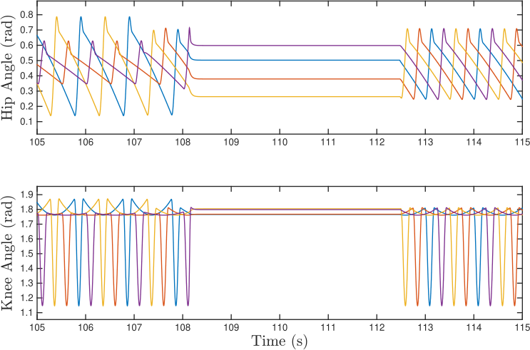
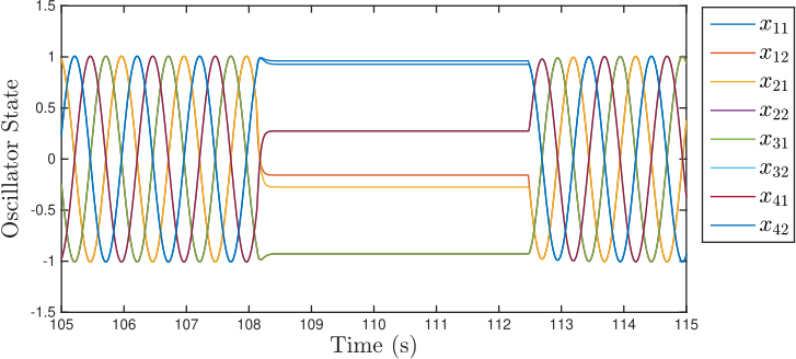
Four coupled oscillators coordinate a four-beat amble on MIT Cheetah, with filtered speed and turning commands. Each leg’s transformation system drives three joints. In the illustrated run, inhibition activates at 108.3 seconds and is removed at 112.4 seconds, stopping and restoring the coordinated oscillations. Body-feedback torques assist balance but are outside the primitive-level proof.
Figure 4: SI-DMPs are applied to provide rhythmic oscillations for a four-beat amble gait.Equations 25–28
(25)
(26)
(27)
(28)
Figure 5: Target kinematics for hip and knee joints during an amble gait with Sparsely-Inhibited Rhythmic DMPs.
Figure 6: Andronov-Hopf oscillator with and without switched inhibition. Upon a state entering a region , a strong contracting dynamic is switched, rendering forward invariant and contracting.Figure 7: Canonical states across the addition and removal of sparse inhibition to the DMP network.
6 Discussion
The framework suggests contact-triggered synchronization, distributed inhibitory voting, and hierarchical control. The reported experiments lack contact sensing, and the analysis does not model how limb forces stabilize the body. Robust locomotion on uncertain terrain therefore remains an extension rather than a demonstrated guarantee.
Equation
Appendix A Selected Proofs
The appendix supplies the metric construction and disturbance bound used in the main analysis.
A.1 Proof of Theorem 1
Starting from a rank-deficient metric that contracts transverse directions, the proof separates tangent and transverse differential coordinates. Integral solutions cancel their cross terms and construct a positive-definite metric. The resulting generalized Jacobian has one zero eigenvalue and strictly negative remaining eigenvalues in its symmetric part.
Equations 29–44
(29)
(30)
(31)
(32)
(33)
(34)
(35)
(36)
(37)
(38)
(39)
(40)
(41)
(42)
(43)
(44)
A.2 Disturbed Transverse Contracting Systems
A virtual time-scaled trajectory aligns the nominal flow with a disturbed trajectory. Bounding the derivative of Riemannian distance gives an orbit-tube radius equal to the disturbance bound divided by contraction rate, multiplied by a metric-conditioning factor. The disturbed trajectory must remain in the compact contraction region.
Equations 45–47
(45)
(46)
(47)
52 references
Ajallooeian et al. (2013a)
Ajallooeian, M., Pouya, S., Sproewitz, A., and Ijspeert, A.J.
(2013a).
Central pattern generators augmented with virtual model control for
quadruped rough terrain locomotion.
In IEEEICRA, 3321–3328.
Ajallooeian et al. (2013b)
Ajallooeian, M., van den Kieboom, J., Mukovskiy, A., Giese, M.A., and Ijspeert,
A.J. (2013b).
A general family of morphed nonlinear phase oscillators with
arbitrary limit cycle shape.
Physica D, 263, 41–56.
Barasuol et al. (2013)
Barasuol, V., Buchli, J., Semini, C., Frigerio, M., Pieri, E.R.D., and
Caldwell, D.G. (2013).
A reactive controller framework for quadrupedal locomotion on
challenging terrain.
In IEEEICRA, 2554–2561.
Bizzi et al. (1995)
Bizzi, E., Giszter, S.F., Loeb, E., Mussa-Ivaldi, F.A., and Saltiel, P. (1995).
Modular organization of motor behavior in the frog’s spinal cord.
Trends Neurosci, 18(10), 442–446.
Canter et al. (2016)
Canter, R.G., Penney, J., and Tsai, L.H. (2016).
The road to restoring neural circuits for the treatment of
alzheimer’s disease.
Nature, 539(7628), 187–196.
URLhttp://dx.doi.org/10.1038/nature20412.
Chung and Slotine (2010)
Chung, S.J. and Slotine, J.J. (2010).
On synchronization of coupled hopf-kuramoto oscillators with phase
delays.
In IEEE Conf. on Decision and Control, 3181–3187.
Chung and Dorothy (2010)
Chung, S.J. and Dorothy, M. (2010).
Neurobiologically inspired control of engineered flapping flight.
Journal of Guidance, Control, and Dynamics, 33(2), 440–453.
Dahlquist (1959)
Dahlquist, G. (1959).
Stability and error bounds in the numerical integration of ordinary
sifferential equations.
Trans. Roy. Inst. Tech. Stockholm, 130.
Davison et al. (2016)
Davison, E.N., Dey, B., and Leonard, N.E. (2016).
Synchronization bound for networks of nonlinear oscillators.
In 54th Annual Allerton Conferecence on Communication, COntrol
and Computing.
Desoer and Haneda (1972)
Desoer, C. and Haneda, H. (1972).
The measure of a matrix as a tool to analyze computer algorithms for
circuit analysis.
IEEE Transactions on Circuit Theory, 19(5), 480–486.
10.1109/TCT.1972.1083507.
Gérard and Slotine (2006)
Gérard, L. and Slotine, J.J. (2006).
Neuronal networks and controlled symmetries, a generic framework.
eprint arXiv:q-bio/0612049.
Ijspeert (2008)
Ijspeert, A.J. (2008).
Central pattern generators for locomotion control in animals and
robots: A review.
Neural Networks, 21(4), 642 – 653.
Ijspeert et al. (2012)
Ijspeert, A.J., Nakanishi, J., Hoffmann, H., Pastor, P., and Schaal, S. (2012).
Dynamical movement primitives: Learning attractor models for motor
behaviors.
Neural Computation, 25(2), 328–373.
Ijspeert et al. (2002)
Ijspeert, A.J., Nakanishi, J., and Schaal, S. (2002).
Learning attractor landscapes for learning motor primitives.
In Advances in NIPS 15, 1547–1554. MIT Press.
Khansari-Zadeh and Billard (2011)
Khansari-Zadeh, S. and Billard, A. (2011).
Learning stable nonlinear dynamical systems with gaussian mixture
models.
IEEE Trans. on Robotics, 27(5), 943–957.
Leonov et al. (1996)
Leonov, G.A., Burkin, I.M., and Shepeljavyi, A.I. (1996).
Frequency Methods in Oscillation Theory, volume 357 of
Mathematics and Its Applications.
Springer.
Manchester et al. (2015)
Manchester, I.R., Tang, J.Z., and Slotine, J.J. (2015).
Unifying classical and optimization-based methods for robot tracking
control with control contraction metrics.
In Proceedings of ISRR.
Manchester and Slotine (2014a)
Manchester, I.R. and Slotine, J.J.E. (2014a).
Combination Properties of Weakly Contracting Systems.
ArXiv e-prints.
arXiv:1408.5174.
Manchester and Slotine (2014b)
Manchester, I.R. and Slotine, J.J.E. (2014b).
Transverse contraction criteria for existence, stability, and
robustness of a limit cycle.
Sys. & Control Letters, 63, 32–38.
Manchester and Slotine (2015)
Manchester, I.R. and Slotine, J.E. (2015).
Control contraction metrics: Convex and intrinsic criteria for
nonlinear feedback design.
CoRR, abs/1503.03144.
URLhttp://arxiv.org/abs/1503.03144.
Marder and Bucher (2001)
Marder, E. and Bucher, D. (2001).
Central pattern generators and the control of rhythmic movements.
Current Biology, 11(23), R986 – R996.
Mussa-Ivaldi et al. (1994)
Mussa-Ivaldi, F.A., Giszter, S.F., and Bizzi, E. (1994).
Linear combinations of primitives in vertebrate motor control.
PNAS, 91(16), 7534–7538.
Park et al. (2017)
Park, H.W., Wensing, P.M., and Kim, S. (2017).
High-speed bounding with the mit cheetah 2: Control design and
experiments.
Submitted to Int J Robot Res.
Park et al. (2015)
Park, H.W., Wensing, P., and Kim, S. (2015).
Online planning for autonomous running jumps over obstacles in
high-speed quadrupeds.
In Proc. of RSS.
Pastor et al. (2009)
Pastor, P., Hoffmann, H., Asfour, T., and Schaal, S. (2009).
Learning and generalization of motor skills by learning from
demonstration.
In IEEEICRA, 763–768.
Pfeffer et al. (2013)
Pfeffer, C.K., Xue, M., He, M., Huang, Z.J., and Scanziani, M. (2013).
Inhibition of inhibition in visual cortex: the logic of connections
between molecularly distinct interneurons.
Nat Neurosci, 16(8), 1068–1076.
Pratt et al. (2001)
Pratt, J., Chew, C.M., Torres, A., Dilworth, P., and Pratt, G. (2001).
Virtual model control: An intuitive approach for bipedal locomotion.
Int J Robot Res, 20(2), 129–143.
Ravichandar and Dani (2015)
Ravichandar, H. and Dani, A. (2015).
Learning contracting nonlinear dynamics from human demonstration for
robot motion planning.
In Proceedings of DSCC. ASME.
Rohrer et al. (2004)
Rohrer, B., Fasoli, S., Krebs, H.I., Volpe, B., Frontera, W.R., Stein, J., and
Hogan, N. (2004).
Submovements grow larger, fewer, and more blended during stroke
recovery.
Motor Control, 8(4), 472–483.
Russo et al. (2013)
Russo, G., di Bernardo, M., and Sontag, E.D. (2013).
A contraction approach to the hierarchical analysis and design of
networked systems.
IEEE Transactions on Automatic Control, 58(5), 1328–1331.
10.1109/TAC.2012.2223355.
Russo and Slotine (2011)
Russo, G. and Slotine, J.J.E. (2011).
Symmetries, stability, and control in nonlinear systems and networks.
Phys. Rev. E, 84, 041929.
10.1103/PhysRevE.84.041929.
Schaal (2006)
Schaal, S. (2006).
Dynamic movement primitives-a framework for motor control in humans
and humanoid robotics.
In Adaptive Motion of Animals and Machines, 261–280.
Springer.
Seo et al. (2010)
Seo, K., Chung, S.J., and Slotine, J.J. (2010).
Cpg-based control of a turtle-like underwater vehicle.
Autonomous Robots, 28(3), 247–269.
Singh et al. (2017)
Singh, S., Majumdar, A., Slotine, J.J., and Pavone, M. (2017).
Robust online motion planning via contraction theory and convex
optimization.
In ICRA submission.
Slotine and Lohmiller (2001)
Slotine, J.J. and Lohmiller, W. (2001).
Modularity, evolution, and the binding problem: a view from stability
theory.
Neural Networks, 14(2), 137 – 145.
Tang and Manchester (2014)
Tang, J. and Manchester, I. (2014).
Transverse contraction criteria for stability of nonlinear hybrid
limit cycles.
In IEEE Conf. on Decision and Control (CDC), 31–36.
Tedrake et al. (2010)
Tedrake, R., Manchester, I.R., Tobenkin, M., and Roberts, J.W. (2010).
LQR-trees: Feedback motion planning via sums-of-squares
verification.
Int J Robot Res, 29(8), 1038–1052.
Wang and Slotine (2005)
Wang, W. and Slotine, J.J.E. (2005).
On partial contraction analysis for coupled nonlinear oscillators.
Biological Cybernetics, 92(1), 38–53.
Wensing et al. (2016)
Wensing, P.M., Wang, A., Seok, S., Otten, D., Lang, J., and Kim, S. (2016).
Proprioceptive actuator design in the MIT cheetah: Impact
mitigation and high-bandwidth physical interaction for dynamic legged robots.
Submitted to IEEE Trans. on Robotics.