At a glance
VLAE deliberately splits image information between a global latent code and a local autoregressive decoder. Restricting what the decoder can predict forces the code to retain complementary information, while a learned autoregressive prior improves density estimation. The paper explains latent-variable collapse through bits-back inefficiency, reports image likelihoods and illustrates controllable lossy reconstructions. The result is architecture-dependent representation learning, not guaranteed recovery of human semantics.
1 Introduction
A strong generative likelihood does not uniquely identify a useful representation: different latent structures, or no latent variables at all, can model the same density. Hybrid variational and autoregressive models often ignore their latent code. The proposed solution uses this information preference deliberately by constraining the decoder and improving the latent prior.
2 VAEs do not autoencode in general
The reconstruction interpretation of a VAE is conditional on its decoder and inference model. A sufficiently expressive autoregressive decoder can model observations without using the latent variable; the ELBO need not reward preserving a near-exact reconstruction in the code.
2.1 Technical background
An inference distribution q(z|x) makes the marginal likelihood tractable through a variational lower bound. Its familiar reconstruction-minus-KL form does not require exact reconstruction: a factorized decoder often needs the latent variable to carry inter-pixel dependence, while an expressive decoder can account for some dependence itself. [27]
Equations 1–3–4



2.2 Bits-back coding and information preference
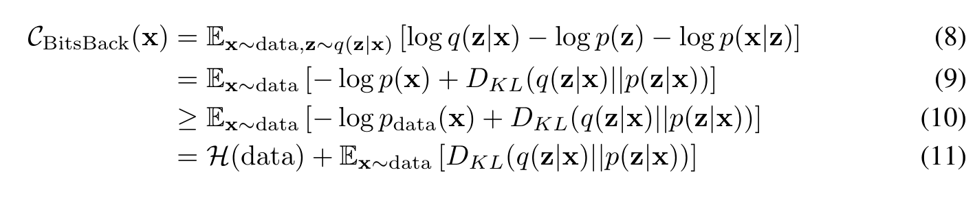
The naive two-part code transmits z and then x given z. Recovering the randomness used to sample z from q subtracts its entropy, so net expected length equals negative ELBO. Relative to ideal data entropy, an approximate posterior adds an inference-gap KL cost. If the decoder can model data without z, discarding z can remove that cost even at a perfectly optimized solution. Thus collapse is not only an optimization accident. Information the decoder can model locally tends to stay local; the rest can pass through z. [20]
Equations 5–8–11


3 Variational Lossy Autoencoder
Two complementary modifications use autoregression: a constrained decoder controls what information must enter the representation, while an autoregressive-flow prior increases modeling flexibility.
3.1 Lossy code via explicit information placement
A PixelCNN decoder with a small receptive field handles local texture but cannot express arbitrary long-range dependence without the latent code. The code is therefore encouraged to capture global structure. Other factorizations could reverse this allocation. The principle is an asymptotic optimization argument; free bits or KL annealing remain useful for actually training the model. The chosen constraint determines what information survives and may discard task-relevant details.
3.2 Learned prior with autoregressive flow
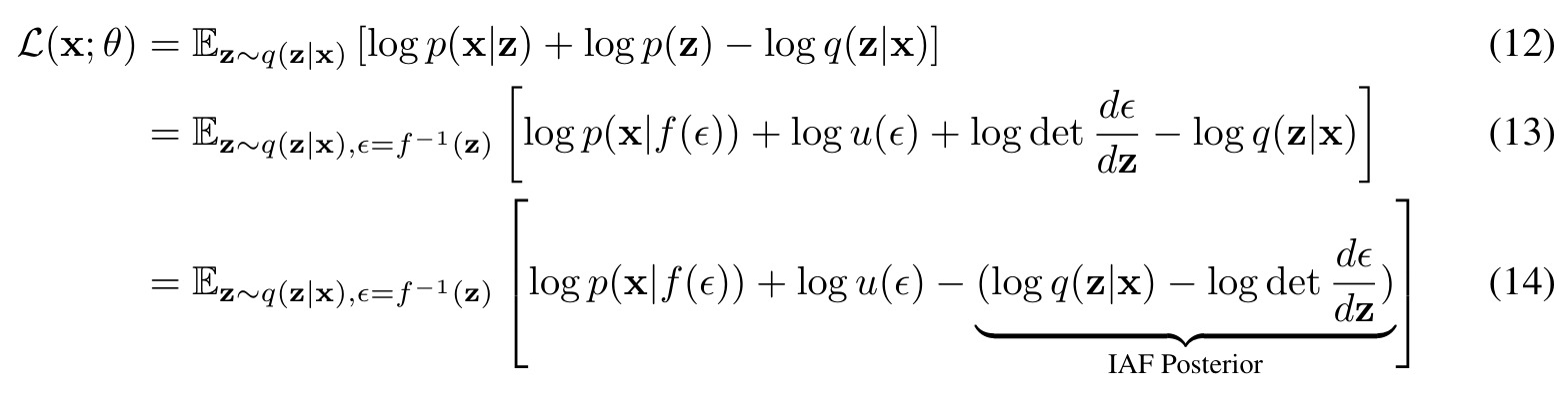
An AF transforms simple noise into a flexible latent prior. Rewriting the objective shows equivalence along the inference path to using an IAF posterior in transformed coordinates, while the generative path gains an extra transformation. Training-time computation under q is comparable, but autoregressive generation remains sequential. This is an expressivity argument, not a claim that every learned posterior becomes exact. [28]
Equation 12–14
4 Experiments
Binary-image experiments use a shared architecture on 28×28 MNIST, OMNIGLOT and Caltech-101 silhouettes, with a six-layer local PixelCNN decoder and an AF prior. Marginal negative log likelihood is estimated with 4,096 importance samples. Hyperparameters are tuned on static MNIST, then reused on the other datasets unless fine-tuning is explicitly marked.
4.1 Lossy compression
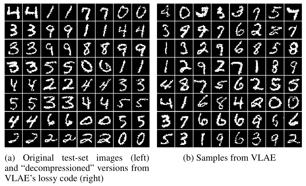
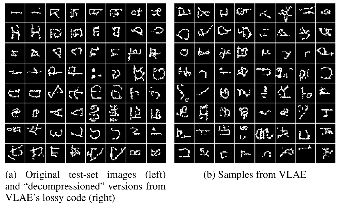
On static MNIST, the latent KL averages 13.3 nats or 19.2 bits, compared with 37.3 bits for the corresponding factorized-decoder VAE. Decoding preserves broad digit structure while regenerating local details. OMNIGLOT examples sometimes lose semantic identity because meaningful details fit inside the local window. A lower latent rate is therefore not automatically a better task representation.
4.2 Density estimation
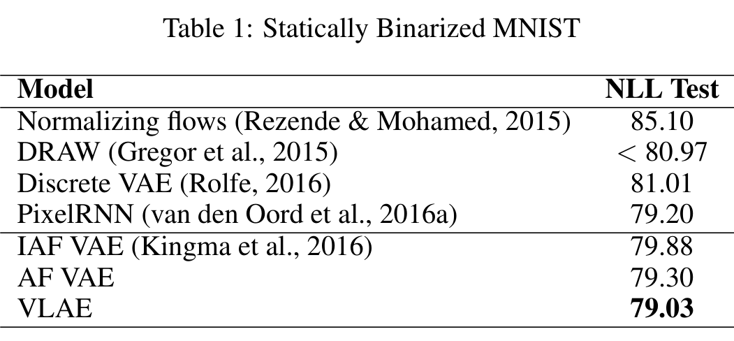
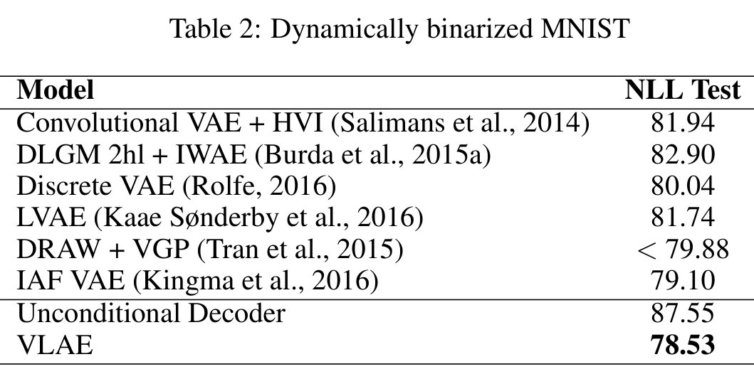
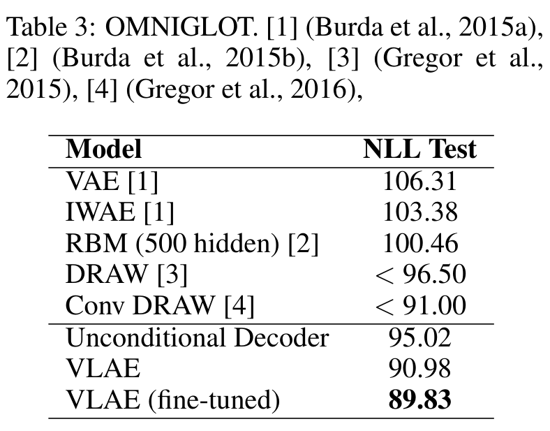
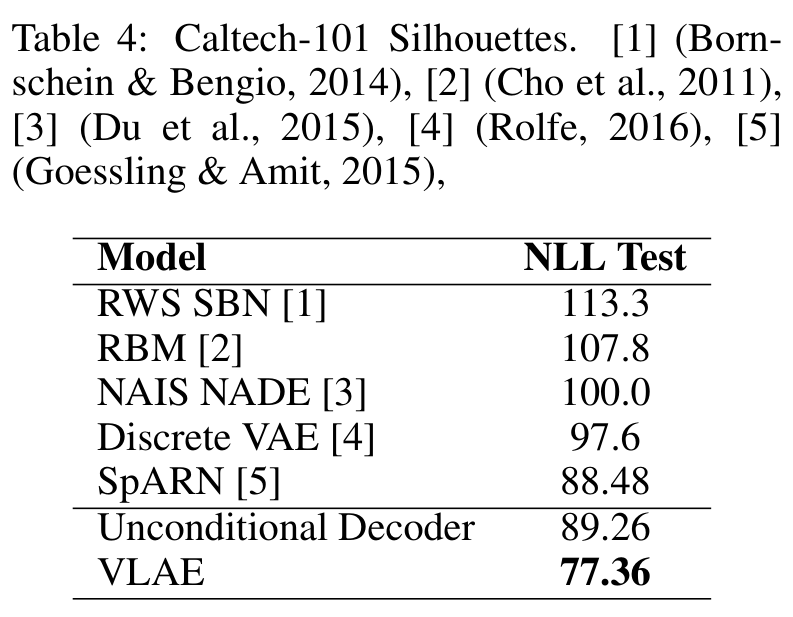
Replacing the IAF posterior with an AF prior improves static-MNIST NLL from 79.88 to 79.30; adding the local decoder yields 79.03. Reported VLAE NLL is 78.53 on dynamic MNIST, 90.98 on OMNIGLOT and 77.36 on Caltech-101; separate OMNIGLOT tuning gives 89.83. The authors compare selected contemporary baselines, with inequalities and dataset-specific evaluation conventions retained in the tables. Likelihood gains do not independently evaluate downstream representation quality.
4.3 Natural images: CIFAR10
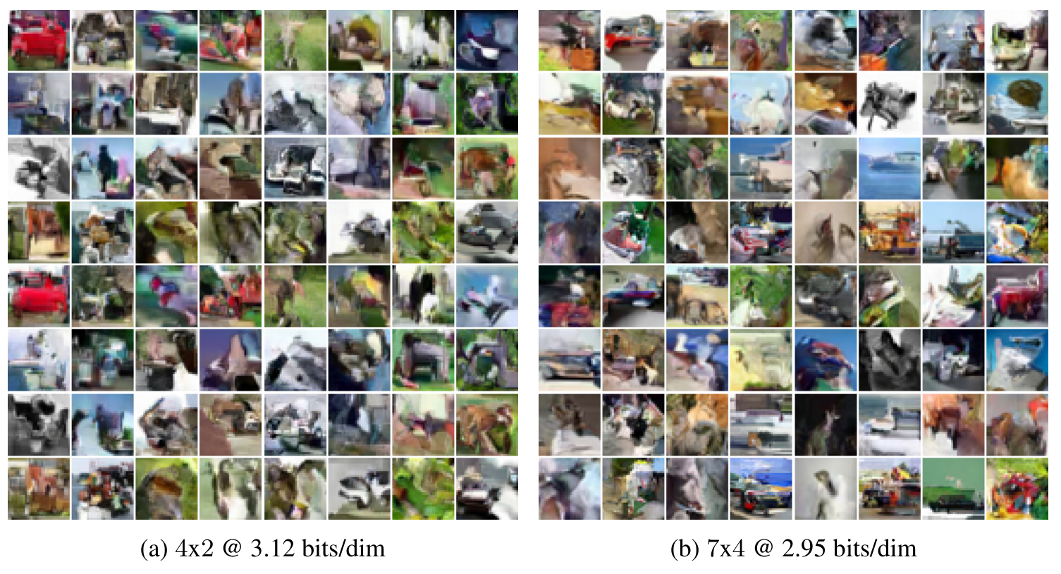
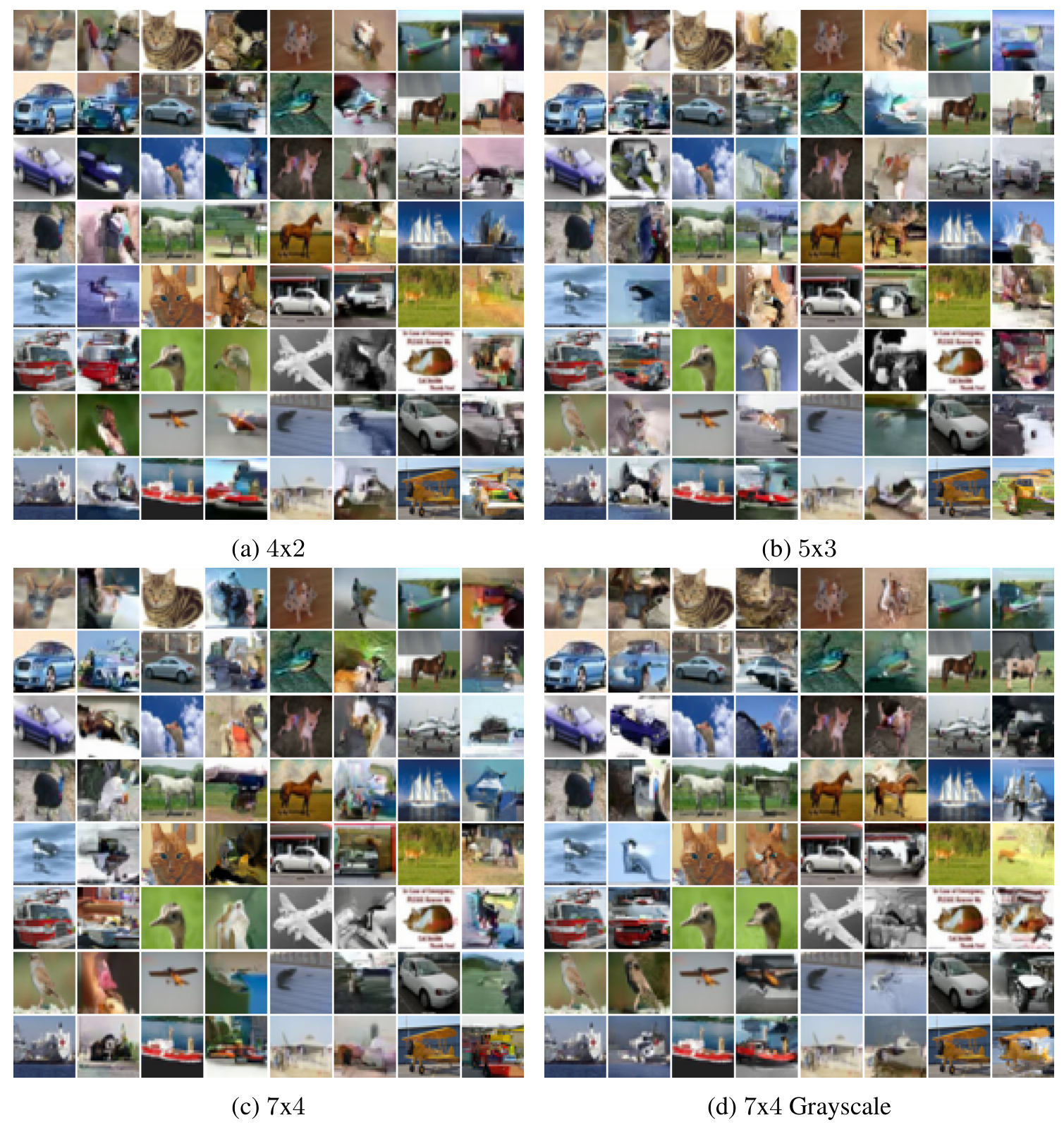
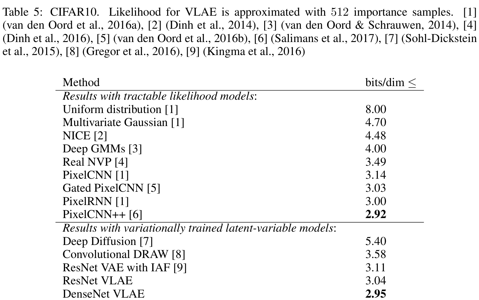
DenseNet components reduce overfitting relative to the tested ResNet version. With 512 importance samples, DenseNet VLAE reports 2.95 bits/dimension, versus 3.04 for ResNet VLAE and 2.92 for the listed PixelCNN++ comparator. Enlarging the decoder receptive field shifts more structure out of the latent code. Conditioning the local decoder on grayscale neighbors forces the latent code to carry more color, producing recognizable examples without demonstrating a general semantic disentanglement guarantee.
5 Related work
The work combines variational inference, autoregressive image modeling and lossy latent representations. PixelVAE concurrently combines latent variables with a PixelCNN decoder; conceptual-compression models use latent hierarchies. The distinguishing proposal here is to control retained information through decoder factorization and to use an explicit autoregressive-flow prior. [18]
6 Conclusion
Decoder restrictions and learned priors provide a principled way to trade local generation against latent information. Benefits in the selected image experiments come with slower sequential generation. Extension to audio/video and task-specific representations is proposed rather than experimentally established.
Appendix A. Binary-image experimental setup
The ResNet encoder/decoder produces four conditioning feature maps concatenated with the binary image for a small masked PixelCNN. Six masked convolutional layers use tied weights for static MNIST to reduce overfitting; additional 1×1 blocks increase capacity. The latent dimension is 64. Four mean-only AF steps use three-layer MADE networks with 640 hidden units. Training uses Adamax at 0.002, 0.01 nats per data dimension of free bits, weight normalization and Polyak averaging with decay 0.998. Validation chooses settings before the final train-plus-validation fit.
Appendix B. CIFAR10 experimental setup
Latents comprise sixteen 8×8 maps. Six autoregressive flows use two-layer PixelCNNs with 128 maps and alternate ordering. ResNet and DenseNet encoders/decoders combine residual/dense blocks and stride-two convolutions. The conditional PixelCNN++ decoder is shallow and wide with 64-map gated blocks. Tested receptive fields are 4×2, 5×3 and 7×4; grayscale uses 0.299R+0.587G+0.114B. The best density result uses 7×4 neighborhoods.
Appendix C. Soft free bits
Hard free bits stop penalizing each latent group below a chosen information allowance, but have a sharp transition. Soft free bits instead scale the KL penalty by an adaptive coefficient γ. If KL exceeds the target by the chosen threshold, increase γ; if it falls below target, decrease γ. The authors use a 5% threshold and 10% multiplicative adjustments. This is a training heuristic to encourage information use, not a changed probabilistic model.
Equations C.1–C.2


Appendix D. Autoregressive decoder without autoregressive prior
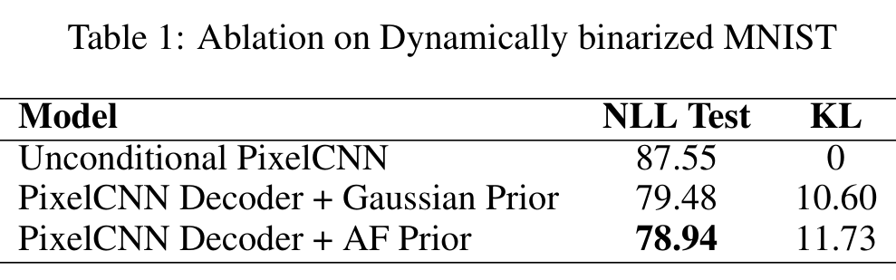
An ablation on dynamic MNIST compares the same local decoder alone, with a Gaussian latent prior, and with an AF prior. NLL improves 87.55 → 79.48 → 78.94, while latent KL increases 0 → 10.60 → 11.73. These ablation values differ from the final main-table recipe; they isolate the benefit of adding latent variables and then a more expressive prior.
Appendix E. CIFAR10 generated samples
The final figure shows unconditional samples from the 4×2 and 7×4 receptive-field models, labeled 3.12 and 2.95 bits/dimension. These illustrate model output rather than an additional quantitative perceptual-quality evaluation.