At a glance
ResNet makes depth easier to optimize by learning a residual correction and adding the input through a shortcut. A 152-layer network improves ImageNet classification while using less computation than VGG; an ensemble reaches 3.57% top-five test error. The same representations improve detection and localization. Very deep networks can still overfit: easier optimization does not guarantee better generalization.
1 Introduction
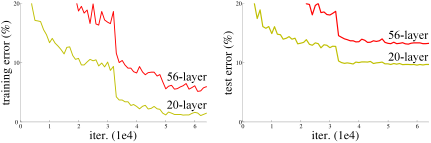
Adding layers to a plain network can increase training error even when initialization and normalization prevent early gradient failure. This is an optimization problem: a deeper network could reproduce a shallower one if its extra layers learned identity maps. Residual blocks make that solution easy by learning a correction to an identity shortcut. Matched plain/residual comparisons isolate the value of this parameterization.
2 Related Work
Residual encodings and multiscale numerical solvers motivate learning deviations from a reference. Earlier networks also used shortcuts, auxiliary classifiers, and gates. ResNet uses an always-open identity path with no learned gating parameters; the residual branch supplies changes to the carried representation.
3 Deep Residual Learning
3.1 Residual Learning
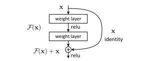
Instead of directly approximating a desired mapping, the stacked layers approximate its difference from the input. The hypothesis is that optimizing a small perturbation around identity is easier than constructing identity through nonlinear layers. Smaller measured residual responses support this interpretation, but are empirical evidence rather than a general optimization proof.
3.2 Identity Mapping by Shortcuts
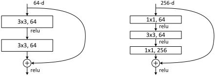
A block adds its input to a two- or three-layer residual function, then applies ReLU. Equal-dimensional shortcuts are identities. When spatial or channel dimensions change, zero padding or a learned projection aligns the two branches. The projection is needed only at those transitions; making every shortcut learned brings little benefit in these experiments.
Equations 1–2
| (1) |
| (2) |
3.3 Network Architectures
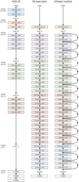
The 18- and 34-layer models use pairs of 3 × 3 convolutions. Deeper models use bottlenecks: a 1 × 1 channel reduction, a 3 × 3 convolution, and a 1 × 1 expansion. Spatial downsampling doubles channel width; global average pooling precedes classification. The 152-layer model requires 11.3 billion multiply-add operations, below VGG-19’s 19.6 billion.
| layer name | output size | 18-layer | 34-layer | 50-layer | 101-layer | 152-layer |
| conv1 | 112112 | 77, 64, stride 2 | ||||
| conv2_x | 5656 | 33 max pool, stride 2 | ||||
| 2 | 3 | 3 | 3 | 3 | ||
| conv3_x | 2828 | 2 | 4 | 4 | 4 | 8 |
| conv4_x | 1414 | 2 | 6 | 6 | 23 | 36 |
| conv5_x | 77 | 2 | 3 | 3 | 3 | 3 |
| 11 | average pool, 1000-d fc, softmax | |||||
| FLOPs | 1.8 | 3.6 | 3.8 | 7.6 | 11.3 | |
3.4 Implementation
ImageNet training uses random scale and crop augmentation, horizontal flips, color augmentation, batch normalization, and SGD with momentum 0.9. The batch size is 256, initial learning rate 0.1, and weight decay 0.0001. Models train from scratch without dropout. Comparisons use ten crops; the strongest results average fully convolutional predictions across scales.
4 Experiments
4.1 ImageNet Classification
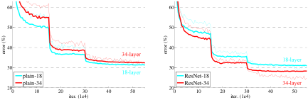
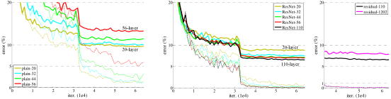
On ImageNet, the 34-layer plain network trains worse than the 18-layer version; residual shortcuts reverse that trend. Identity shortcuts improve the 34-layer baseline by 3.5 percentage points in top-one error without extra parameters. Bottleneck networks improve with depth through 152 layers, reaching 4.49% top-five validation error with multiscale testing. The six-model ensemble reaches 3.57% top-five test error and wins the 2015 classification challenge.
| plain | ResNet | |
|---|---|---|
| 18 layers | 27.94 | 27.88 |
| 34 layers | 28.54 | 25.03 |
| model | top-1 err. | top-5 err. |
|---|---|---|
| VGG-16 [41] | 28.07 | 9.33 |
| GoogLeNet [44] | - | 9.15 |
| PReLU-net [13] | 24.27 | 7.38 |
| plain-34 | 28.54 | 10.02 |
| ResNet-34 A | 25.03 | 7.76 |
| ResNet-34 B | 24.52 | 7.46 |
| ResNet-34 C | 24.19 | 7.40 |
| ResNet-50 | 22.85 | 6.71 |
| ResNet-101 | 21.75 | 6.05 |
| ResNet-152 | 21.43 | 5.71 |
4.2 CIFAR-10 and Analysis
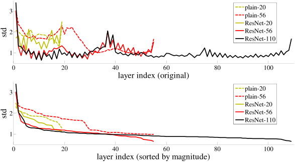
CIFAR-10 models use 6n + 2 layers and identity shortcuts. Residual networks improve as depth grows to 110 layers, with 6.43% test error for the reported best run. Residual branch activations tend to be smaller than plain-network responses. A 1,202-layer model reaches below 0.1% training error but 7.93% test error, consistent with overfitting on this small dataset rather than failed optimization.
| output map size | 3232 | 1616 | 88 |
|---|---|---|---|
| # layers | 1+2 | 2 | 2 |
| # filters | 16 | 32 | 64 |
| method | error (%) | ||
| Maxout [10] | 9.38 | ||
| NIN [25] | 8.81 | ||
| DSN [24] | 8.22 | ||
| # layers | # params | ||
| FitNet [35] | 19 | 2.5M | 8.39 |
| Highway [42, 43] | 19 | 2.3M | 7.54 (7.720.16) |
| Highway [42, 43] | 32 | 1.25M | 8.80 |
| ResNet | 20 | 0.27M | 8.75 |
| ResNet | 32 | 0.46M | 7.51 |
| ResNet | 44 | 0.66M | 7.17 |
| ResNet | 56 | 0.85M | 6.97 |
| ResNet | 110 | 1.7M | 6.43 (6.610.16) |
| ResNet | 1202 | 19.4M | 7.93 |
4.3 Object Detection on PASCAL and MS COCO
Replacing VGG-16 with ResNet-101 in the same Faster R-CNN detector raises PASCAL detection accuracy and increases COCO mean average precision from 21.2% to 27.2% under the stricter overlap-averaged metric. This six-point gain comes from the representation, before the competition-specific improvements in the appendices.
Appendix A Object Detection Baselines
The detector shares convolutional features through the fourth stage, applies region pooling, then uses the final residual stage for each region. ImageNet batch-normalization statistics remain fixed during detection fine-tuning. The proposal network supplies 300 regions. PASCAL uses the standard combined training splits; COCO training uses 80,000 images and evaluates 40,000 validation images. The controlled comparison keeps detection machinery constant across backbones.
Appendix B Object Detection Improvements
Competition models add a second box-refinement pass, a global image-context feature, and multiscale testing. Three-network ensembling improves both proposals and classification, reaching 37.4% COCO precision averaged over overlap thresholds. Fine-tuning the improved model on PASCAL reaches 85.6% and 83.8% on the 2007 and 2012 test sets. On ImageNet detection, the three-model ensemble reaches 62.1% mean average precision. These gains include the added detection procedures, beyond the backbone-only comparison.
| training data | COCO train | COCO trainval | ||
|---|---|---|---|---|
| test data | COCO val | COCO test-dev | ||
| mAP | @.5 | @[.5, .95] | @.5 | @[.5, .95] |
| baseline Faster R-CNN (VGG-16) | 41.5 | 21.2 | ||
| baseline Faster R-CNN (ResNet-101) | 48.4 | 27.2 | ||
| +box refinement | 49.9 | 29.9 | ||
| +context | 51.1 | 30.0 | 53.3 | 32.2 |
| +multi-scale testing | 53.8 | 32.5 | 55.7 | 34.9 |
| ensemble | 59.0 | 37.4 | ||
| system | net | data | mAP | areo | bike | bird | boat | bottle | bus | car | cat | chair | cow | table | dog | horse | mbike | person | plant | sheep | sofa | train | tv |
|---|---|---|---|---|---|---|---|---|---|---|---|---|---|---|---|---|---|---|---|---|---|---|---|
| baseline | VGG-16 | 07+12 | 73.2 | 76.5 | 79.0 | 70.9 | 65.5 | 52.1 | 83.1 | 84.7 | 86.4 | 52.0 | 81.9 | 65.7 | 84.8 | 84.6 | 77.5 | 76.7 | 38.8 | 73.6 | 73.9 | 83.0 | 72.6 |
| baseline | ResNet-101 | 07+12 | 76.4 | 79.8 | 80.7 | 76.2 | 68.3 | 55.9 | 85.1 | 85.3 | 89.8 | 56.7 | 87.8 | 69.4 | 88.3 | 88.9 | 80.9 | 78.4 | 41.7 | 78.6 | 79.8 | 85.3 | 72.0 |
| baseline+++ | ResNet-101 | COCO+07+12 | 85.6 | 90.0 | 89.6 | 87.8 | 80.8 | 76.1 | 89.9 | 89.9 | 89.6 | 75.5 | 90.0 | 80.7 | 89.6 | 90.3 | 89.1 | 88.7 | 65.4 | 88.1 | 85.6 | 89.0 | 86.8 |
| system | net | data | mAP | areo | bike | bird | boat | bottle | bus | car | cat | chair | cow | table | dog | horse | mbike | person | plant | sheep | sofa | train | tv |
|---|---|---|---|---|---|---|---|---|---|---|---|---|---|---|---|---|---|---|---|---|---|---|---|
| baseline | VGG-16 | 07++12 | 70.4 | 84.9 | 79.8 | 74.3 | 53.9 | 49.8 | 77.5 | 75.9 | 88.5 | 45.6 | 77.1 | 55.3 | 86.9 | 81.7 | 80.9 | 79.6 | 40.1 | 72.6 | 60.9 | 81.2 | 61.5 |
| baseline | ResNet-101 | 07++12 | 73.8 | 86.5 | 81.6 | 77.2 | 58.0 | 51.0 | 78.6 | 76.6 | 93.2 | 48.6 | 80.4 | 59.0 | 92.1 | 85.3 | 84.8 | 80.7 | 48.1 | 77.3 | 66.5 | 84.7 | 65.6 |
| baseline+++ | ResNet-101 | COCO+07++12 | 83.8 | 92.1 | 88.4 | 84.8 | 75.9 | 71.4 | 86.3 | 87.8 | 94.2 | 66.8 | 89.4 | 69.2 | 93.9 | 91.9 | 90.9 | 89.6 | 67.9 | 88.2 | 76.8 | 90.3 | 80.0 |
Appendix C ImageNet Localization
Localization uses class-specific proposal scores and box regressors. With ground-truth classes, a single ResNet-101 proposal model reduces center-crop localization error to 13.3%. Dense multiscale proposals and a region-centric R-CNN refinement stage yield 10.6% top-five localization error with predicted classes. Ensembling reaches 9.0% on the test set. Region-centric training avoids near-identical proposals dominating an image-based minibatch.
|
|
testing |
|
|
| ||||||||||
|---|---|---|---|---|---|---|---|---|---|---|---|---|---|---|---|
| VGG’s [41] | VGG-16 | 1-crop | 33.1 [41] | ||||||||||||
| RPN | ResNet-101 | 1-crop | 13.3 | ||||||||||||
| RPN | ResNet-101 | dense | 11.7 | ||||||||||||
| RPN | ResNet-101 | dense | ResNet-101 | 14.4 | |||||||||||
| RPN+RCNN | ResNet-101 | dense | ResNet-101 | 10.6 | |||||||||||
| RPN+RCNN | ensemble | dense | ensemble | 8.9 |