At a glance
Deep Speech 2 combines convolutional and recurrent networks with CTC training for English and Mandarin transcription. Better optimization, more labeled data, and faster GPU systems improve recognition and make large experiments practical. It matches or exceeds the tested human workers on some benchmarks, but remains worse on several accents and noisy conditions.
1 Introduction
The contribution spans models, data, and systems: deeper speech networks, about 12,000 English and 9,400 Mandarin training hours, and synchronized multi-GPU training that finishes in days. A separate streaming deployment configuration trades a small accuracy loss for low compute latency. “End-to-end” here still includes an external language model during decoding.
2 Related Work
The work builds on neural acoustic models, recurrent and convolutional recognition, CTC, and earlier Deep Speech. Unlike pipelines that require frame-level alignment labels or phonetic pretraining, its acoustic model trains from audio–transcript pairs. Data augmentation and recognition-assisted dataset cleaning also draw on prior work.
3 Model Architecture
Deeper networks require better optimization and more computation. The paper studies sequence-wise batch normalization, a short-first training curriculum, frequency convolutions, temporal strides, and streaming-compatible recurrence. Ablations separate several of these effects.
3.1 Preliminaries
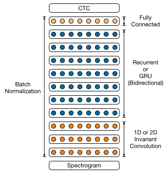
A power-normalized spectrogram passes through convolutional, recurrent, and fully connected layers to predict characters plus a blank symbol. CTC sums over possible alignments between audio frames and transcription. English is evaluated with WER, Mandarin with CER; most reported recognition results include language-model decoding.
Equations 1–5
| (1) |
| (2) | ||||
| (3) |
| (4) |
| (5) |
3.2 Batch Normalization for Deep RNNs
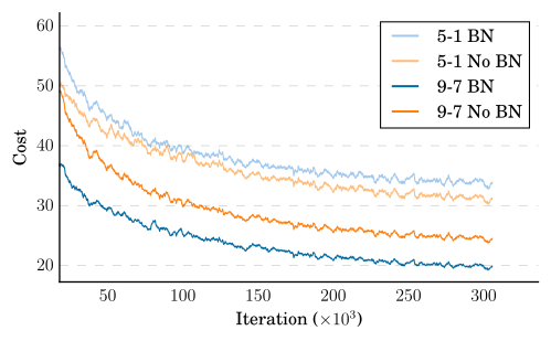
Batch normalization acts on input-to-hidden transformations using statistics pooled over sequences and the minibatch, leaving recurrent contributions outside that normalization. It improves deeper networks but can hurt the shallowest one. Deployment uses running training statistics rather than recomputing normalization from one utterance.
Equations 6–8
| (6) |
| (7) |
| (8) |
| Architecture | Hidden Units | Train | Dev | ||||||
|---|---|---|---|---|---|---|---|---|---|
| Baseline | BatchNorm | Baseline | BatchNorm | ||||||
| 1 RNN, 5 total | 2400 | 10.55 | 11.99 | 13.55 | 14.40 | ||||
| 3 RNN, 5 total | 1880 | 9.55 | 8.29 | 11.61 | 10.56 | ||||
| 5 RNN, 7 total | 1510 | 8.59 | 7.61 | 10.77 | 9.78 | ||||
| 7 RNN, 9 total | 1280 | 8.76 | 7.68 | 10.83 | 9.52 | ||||
3.3 SortaGrad
SortaGrad processes shorter utterances first only during the first epoch, then returns to randomized minibatches. It reduces early optimization instability and complements batch normalization. Utterance length is a difficulty heuristic, not an externally labeled curriculum.
Equation 9
| (9) |
| Train | Dev | |||||||
|---|---|---|---|---|---|---|---|---|
| Baseline | BatchNorm | Baseline | BatchNorm | |||||
| Not Sorted | 10.71 | 8.04 | 11.96 | 9.78 | ||||
| Sorted | 8.76 | 7.68 | 10.83 | 9.52 | ||||
3.4 Comparison of simple RNNs and GRUs
At roughly equal parameter counts, GRUs outperform simple recurrent units across the tested depths. With larger models and a fixed computational budget, deeper simple RNNs become competitive or better. The paper’s GRU variant moves the reset operation after the recurrent matrix multiplication to combine computations efficiently.
Equation 10
| (10) | ||||
| Architecture | Simple RNN | GRU |
|---|---|---|
| 5 layers, 1 Recurrent | 14.40 | 10.53 |
| 5 layers, 3 Recurrent | 10.56 | 8.00 |
| 7 layers, 5 Recurrent | 9.78 | 7.79 |
| 9 layers, 7 Recurrent | 9.52 | 8.19 |
3.5 Frequency Convolutions
Convolutions over both frequency and time improve robustness to spectral variation, especially in noisy audio. Moving from one temporal convolution to three two-dimensional convolutions reduces noisy-development WER by 23.9% relative in the reported ablation. Convolutions come before recurrent layers so frequency structure remains available.
| Architecture | Channels | Filter dimension | Stride | Regular Dev | Noisy Dev |
|---|---|---|---|---|---|
| 1-layer 1D | 1280 | 11 | 2 | 9.52 | 19.36 |
| 2-layer 1D | 640, 640 | 5, 5 | 1, 2 | 9.67 | 19.21 |
| 3-layer 1D | 512, 512, 512 | 5, 5, 5 | 1, 1, 2 | 9.20 | 20.22 |
| 1-layer 2D | 32 | 41x11 | 2x2 | 8.94 | 16.22 |
| 2-layer 2D | 32, 32 | 41x11, 21x11 | 2x2, 2x1 | 9.06 | 15.71 |
| 3-layer 2D | 32, 32, 96 | 41x11, 21x11, 21x11 | 2x2, 2x1, 2x1 | 8.61 | 14.74 |
3.6 Striding
Larger temporal strides shorten recurrent sequences and reduce memory and work. English character outputs become too dense for aggressive strides, so the model predicts non-overlapping character bigrams, with single-character leftovers and spaces. This shortens the output sequence while preserving a deterministic text mapping.
| Dev no LM | Dev LM | |||||||||||
| Stride | Unigrams | Bigrams | Unigrams | Bigrams | ||||||||
| 2 | 14.93 | 14.56 | 9.52 | 9.66 | ||||||||
| 3 | 15.01 | 15.60 | 9.65 | 10.06 | ||||||||
| 4 | 18.86 | 14.84 | 11.92 | 9.93 | ||||||||
3.7 Row Convolution and Unidirectional Models
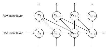
Bidirectional recurrence needs the whole utterance. For streaming, forward-only recurrent layers feed a row convolution that uses a bounded future window. This separates most incremental computation from the limited lookahead required near the output.
Equation 11
| (11) |
3.8 Language Model
A five-gram language model supplements the acoustic network: word-level for English, character-level for Mandarin. Beam search combines acoustic log probability, language-model log probability, and an insertion term. Deeper networks need less relative help from the external model, but the reported gains remain substantial.
Equation 12
| (12) |
| Language | Architecture | Dev no LM | Dev LM | ||||
|---|---|---|---|---|---|---|---|
| English | 5-layer, 1 RNN | 27.79 | 14.39 | ||||
| English | 9-layer, 7 RNN | 14.93 | 9.52 | ||||
| Mandarin | 5-layer, 1 RNN | 9.80 | 7.13 | ||||
| Mandarin | 9-layer, 7 RNN | 7.55 | 5.81 | ||||
3.9 Adaptation to Mandarin
The Mandarin system directly predicts about 6,000 characters, including Roman letters, without a separate pronunciation or tone model. Decoding uses a character language model and insertion term. Its lower character rate also makes temporal striding easier than in English.
4 System Optimizations
The custom training system combines optimized recurrent computation, communication, CTC, and allocation. These engineering changes make architecture and data experiments feasible at the reported scale.
4.1 Scalability and Data-Parallelism
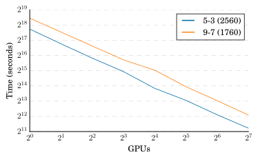
Synchronous data-parallel training averages gradients across GPUs. A ring all-reduce implementation reduces unnecessary memory copies and improves communication, especially within an eight-GPU node. The scaling experiment keeps examples per GPU fixed, so global minibatch size grows; it is a weak-scaling comparison, not constant-batch scaling.
| GPU | OpenMPI | Our | Performance | ||||||
|---|---|---|---|---|---|---|---|---|---|
| all-reduce | all-reduce | Gain | |||||||
| 4 | 55359.1 | 2587.4 | 21.4 | ||||||
| 8 | 48881.6 | 2470.9 | 19.8 | ||||||
| 16 | 21562.6 | 1393.7 | 15.5 | ||||||
| 32 | 8191.8 | 1339.6 | 6.1 | ||||||
| 64 | 1395.2 | 611.0 | 2.3 | ||||||
| 128 | 1602.1 | 422.6 | 3.8 | ||||||
4.2 GPU implementation of CTC loss function
Moving CTC loss and gradient computation onto GPUs avoids large CPU transfers and speeds that component by 28.9 times for English and 12.5 times for Mandarin in the reported tests. End-to-end training improves by a smaller 10–20%, since CTC is only one component.
| Language | Architecture | CPU CTC Time | GPU CTC Time | Speedup |
|---|---|---|---|---|
| English | 5-layer, 3 RNN | 5888.12 | 203.56 | 28.9 |
| Mandarin | 5-layer, 3 RNN | 1688.01 | 135.05 | 12.5 |
4.3 Memory allocation
A custom allocator subdivides preallocated blocks to avoid repeated operating-system allocation overhead. Activations dominate memory use; exceptional long utterances can spill into mapped host memory at reduced bandwidth. This reduces failures without making host access as fast as local GPU memory.
5 Training Data
English training combines public and internal corpora for 11,940 hours and eight million utterances. Mandarin uses 9,400 hours and eleven million utterances, including read and spontaneous speech. Table 9 retains the English corpus breakdown.
| Dataset | Speech Type | Hours |
|---|---|---|
| WSJ | read | 80 |
| Switchboard | conversational | 300 |
| Fisher | conversational | 2000 |
| LibriSpeech | read | 960 |
| Baidu | read | 5000 |
| Baidu | mixed | 3600 |
| Total | 11940 |
5.1 Dataset Construction
An existing bidirectional CTC recognizer aligns long audio with noisy transcripts; stretches of blank predictions provide segmentation boundaries. A classifier filters likely bad alignments using recognition costs and length ratios. On the described English subset, filtering lowers transcript WER from 17% to 5% while retaining over half the examples.
Equation 13
| (13) |
5.2 Data Augmentation
Noise is added to 40% of randomly selected training utterances, using a large pool of audio sources. Too little augmentation weakens noise robustness; too much makes optimization harder.
5.3 Scaling Data
Increasing training data improves regular and noisy development WER across the tested subsets. The authors describe an approximate power-law trend and hypothesize that diversity of speakers and contexts matters alongside total hours. The experiment varies randomly sampled data volume, so it does not directly isolate that diversity hypothesis.
| Fraction of Data | Hours | Regular Dev | Noisy Dev | ||||||
|---|---|---|---|---|---|---|---|---|---|
| 1% | 120 | 29.23 | 50.97 | ||||||
| 10% | 1200 | 13.80 | 22.99 | ||||||
| 20% | 2400 | 11.65 | 20.41 | ||||||
| 50% | 6000 | 9.51 | 15.90 | ||||||
| 100% | 12000 | 8.46 | 13.59 | ||||||
6 Results
Models train with momentum, gradient clipping, and scheduled learning-rate decay; the best held-out development checkpoint is evaluated. English and Mandarin use different beam widths and metrics. Results span public and internal datasets rather than one uniform test distribution.
6.1 English
The strongest English model has three frequency–time convolution layers and seven bidirectional recurrent layers. Human comparisons use the better of two crowd-worker transcriptions per clip, with repeated listening allowed. These workers and short-clip conditions define the comparison; the numbers are not a universal human-performance ceiling.
6.1.1 Model Size
Recognition improves up to the tested 100-million-parameter size. The selected simple-RNN model reduces WER on an internal mixed-condition test from 24.01% to 13.59%. Table 11’s caption incorrectly says all models have approximately 35 million parameters despite listing 18–100 million; its explicit row values and accompanying discussion describe the actual size comparison.
| Model size | Model type | Regular Dev | Noisy Dev | ||||
|---|---|---|---|---|---|---|---|
| GRU | 10.59 | 21.38 | |||||
| GRU | 9.06 | 17.07 | |||||
| GRU | 8.54 | 15.98 | |||||
| RNN | 8.44 | 15.09 | |||||
| GRU | 7.78 | 14.17 | |||||
| RNN | 7.73 | 13.06 | |||||
6.1.2 Read Speech
On clean read speech, the model beats the measured workers on three of four test sets. It remains slightly worse on LibriSpeech test-other, at 13.25% versus 12.69% WER. These results concern read speech and do not remove the harder accent and noise gaps below.
6.1.3 Accented Speech
VoxForge tests cover American–Canadian, Commonwealth, European, and Indian accents. Deep Speech 2 substantially improves its predecessor but stays worse than the measured human results in every row, with the Indian-accent comparison close. Training breadth remains a limitation.
6.1.4 Noisy Speech
Single-channel CHiME evaluation shows major improvement over the earlier system but substantial remaining human gaps: real-noise WER is 21.79% versus 11.84%, and simulated-noise WER 45.05% versus 31.33%. Multi-channel enhancement is not used in these comparisons.
| Noisy Speech | |||
|---|---|---|---|
| Test set | DS1 | DS2 | Human |
| CHiME eval clean | 6.30 | 3.34 | 3.46 |
| CHiME eval real | 67.94 | 21.79 | 11.84 |
| CHiME eval sim | 80.27 | 45.05 | 31.33 |
6.2 Mandarin
Deeper normalized recurrent models with frequency convolutions reduce internal Mandarin test CER from 15.41% to 7.93%. Separate human comparisons use small samples of 100 and 250 short queries; their results support those settings, not a broad claim about all Mandarin speech.
| Architecture | Dev | Test |
|---|---|---|
| 5-layer, 1 RNN | 7.13 | 15.41 |
| 5-layer, 3 RNN | 6.49 | 11.85 |
| 5-layer, 3 RNN + BatchNorm | 6.22 | 9.39 |
| 9-layer, 7 RNN + BatchNorm + 2D conv | 5.81 | 7.93 |
7 Deployment
Deployment replaces full-utterance operations with adaptive input normalization, forward recurrence, bounded lookahead, and cheaper decoding. Reported latency starts at the end of the utterance and excludes Internet transport; it is not time to the first partial transcript.
7.1 Batch Dispatch
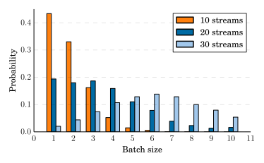
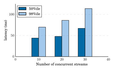
Batch Dispatch eagerly groups ready streams whenever the previous batch finishes. This gains some matrix-multiplication efficiency without waiting to fill a large batch. At ten concurrent streams, the section reports 44 ms median and roughly 70 ms 98th-percentile compute latency; the introduction gives 67 ms for the latter.
7.2 Deployment Optimized Matrix Multiply Kernels
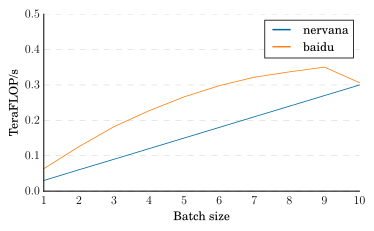
Half-precision inference reduces weight traffic with no measurable recognition loss in these tests. Custom matrix kernels target the very small batches typical of interactive serving, a different regime from large training batches.
7.3 Beam Search
Mandarin beam search considers only enough likely next characters to cover cumulative probability 0.99, capped at forty. This sharply reduces language-model lookups with a reported 0.1–0.3% relative CER cost.
7.4 Results
The deployed Mandarin system reaches 6.10% CER versus 5.81% for the research system on 2,000 held-out utterances. Its five forward recurrent layers, row convolution, half precision, batching, and pruned decoding jointly achieve the stated latency–accuracy tradeoff.
8 Conclusion
Larger datasets and models become useful when optimization and hardware execution scale with them. The paper demonstrates this across two languages and a deployable recognizer, while its own tests still expose sizable accent and noise limitations.
Acknowledgments
The authors acknowledge Baidu’s speech group, Nervana Systems, and NVIDIA for data, numerical kernels, and discussions.
Appendix A Scalability improvements
The appendix details the hardware topology and GPU loss computation underlying the training-speed results.
A.1 Node and cluster architecture
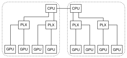
Each node combines two CPUs, eight Titan X GPUs, local data storage, and substantial host memory. GPU placement within PCI root complexes enables faster transfers, and InfiniBand carries gradients between nodes. Replicated local datasets keep input traffic away from the inter-node network.
A.2 GPU Implementation of CTC Loss Function
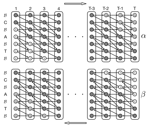
The GPU CTC implementation works in log-probability space and computes whole dynamic-programming columns in parallel, including some invalid entries whose contributions vanish when forward and backward values combine. Sorting labels once groups repeated characters for efficient gradient reductions. Columns remain sequentially dependent, while work within each column is parallel. Figure 9 retains the valid, invalid, and discarded-value layout.