At a glance
Dense prediction needs both precise pixel locations and broad context. Dilated convolutions enlarge the receptive field while preserving feature-map resolution. A small context module improves several segmentation systems; simplifying an inherited image-classification backbone also improves accuracy. The appendix extends the design to urban-scene datasets.
1 Introduction
Pooling-heavy classification networks discard spatial detail that segmentation must later recover. Rather than repeatedly downsample and upsample or process multiple image scales, the proposed context module keeps resolution constant and expands filter spacing. Controlled experiments separate the benefits of this module from structured prediction and extra training data.
2 Dilated Convolutions
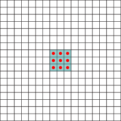
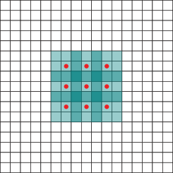
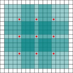
A dilation factor spaces a convolution’s sampling positions without adding filter parameters. Stacking 3 × 3 filters with exponentially increasing dilation gives exponentially larger receptive fields while keeping dense output coverage. This operator has roots in wavelet methods; it is a component of the à trous algorithm, not the algorithm itself.
Equations 1–3
| (1) |
| (2) |
| (3) |
3 Multi-Scale Context Aggregation
The basic context module uses seven 3 × 3 layers with dilations 1, 1, 2, 4, 8, 16, and 1, followed by a 1 × 1 output layer. It keeps one feature map per class and reaches a 67 × 67 receptive field. Identity initialization lets it start by passing predictions through; ordinary random initialization was ineffective here. A larger version adds channels and uses a generalized identity initialization with small noise to break symmetry.
Equation 4
| (4) |
| Layer | 1 | 2 | 3 | 4 | 5 | 6 | 7 | 8 |
|---|---|---|---|---|---|---|---|---|
| Convolution | ||||||||
| Dilation | 1 | 1 | 2 | 4 | 8 | 16 | 1 | 1 |
| Truncation | Yes | Yes | Yes | Yes | Yes | Yes | Yes | No |
| Receptive field | ||||||||
| Output channels | ||||||||
| Basic | ||||||||
| Large | ||||||||
Equation 5
| (5) |


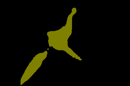



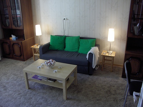
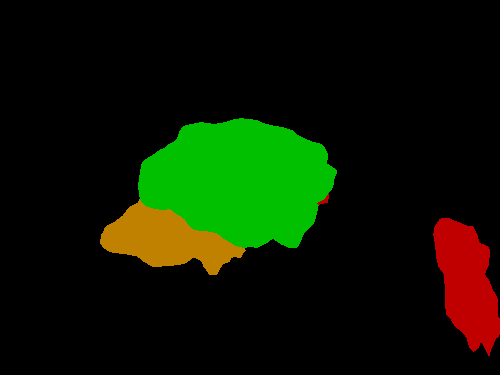
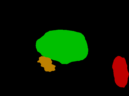
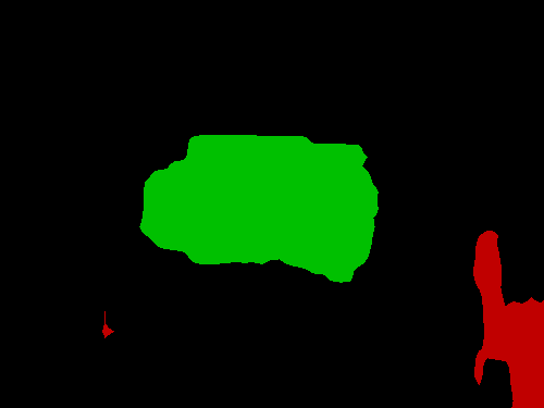
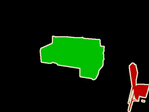
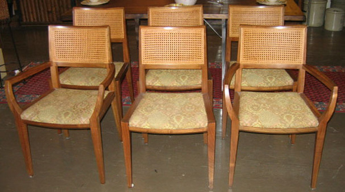




|
aero |
bike |
bird |
boat |
bottle |
bus |
car |
cat |
chair |
cow |
table |
dog |
horse |
mbike |
person |
plant |
sheep |
sofa |
train |
tv |
mean IoU | |
|---|---|---|---|---|---|---|---|---|---|---|---|---|---|---|---|---|---|---|---|---|---|
| FCN-8s | 76.8 | 34.2 | 68.9 | 49.4 | 60.3 | 75.3 | 74.7 | 77.6 | 21.4 | 62.5 | 46.8 | 71.8 | 63.9 | 76.5 | 73.9 | 45.2 | 72.4 | 37.4 | 70.9 | 55.1 | 62.2 |
| DeepLab | 72 | 31 | 71.2 | 53.7 | 60.5 | 77 | 71.9 | 73.1 | 25.2 | 62.6 | 49.1 | 68.7 | 63.3 | 73.9 | 73.6 | 50.8 | 72.3 | 42.1 | 67.9 | 52.6 | 62.1 |
| DeepLab-Msc | 74.9 | 34.1 | 72.6 | 52.9 | 61.0 | 77.9 | 73.0 | 73.7 | 26.4 | 62.2 | 49.3 | 68.4 | 64.1 | 74.0 | 75.0 | 51.7 | 72.7 | 42.5 | 67.2 | 55.7 | 62.9 |
| Our front end | 82.2 | 37.4 | 72.7 | 57.1 | 62.7 | 82.8 | 77.8 | 78.9 | 28 | 70 | 51.6 | 73.1 | 72.8 | 81.5 | 79.1 | 56.6 | 77.1 | 49.9 | 75.3 | 60.9 | 67.6 |
4 Front End
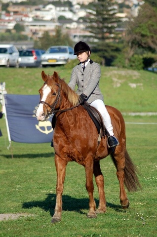
The front end adapts VGG-16 by removing the last two pooling/striding operations and dilating later filters, preserving pretrained weights while increasing output resolution. It also removes intermediate padding and uses reflection padding around the input image. Trained on the standard augmented PASCAL split, this simpler front end reaches 67.6% test mean intersection over union, more than five points above the compared FCN-8s and DeepLab versions.
5 Experiments
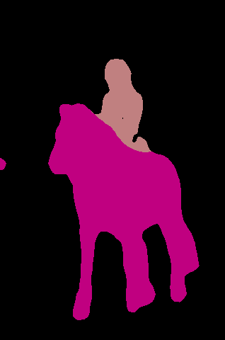
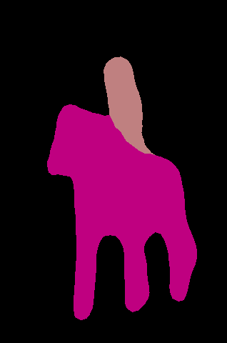
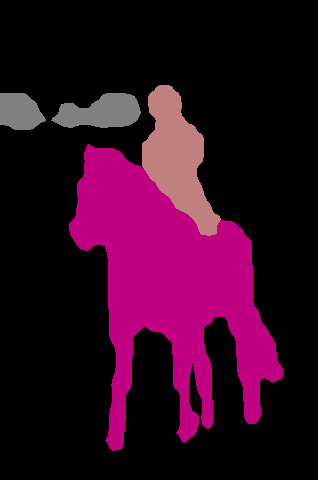
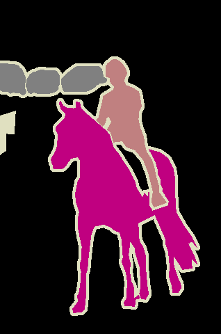
A stronger front end first trains on PASCAL plus matching COCO categories, then fine-tunes on PASCAL alone. It reaches 69.8% validation and 71.3% test mean intersection over union before context or structured prediction. This distinction matters: comparisons must account for the extra training images.
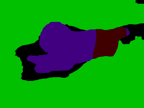
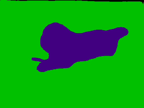
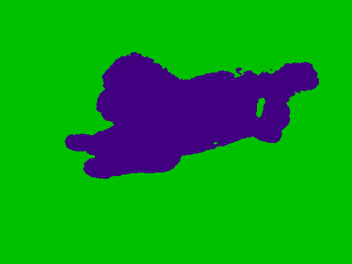
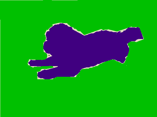
Controlled evaluation of context aggregation.
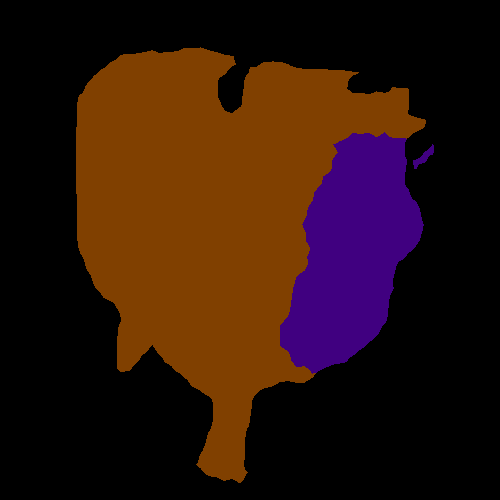
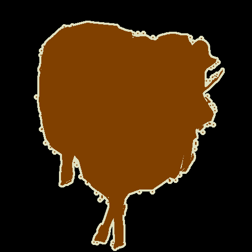
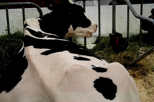
Both context-module sizes improve the front end alone, the front end with a dense conditional random field, and the recurrent conditional-random-field system. The larger module helps more. Its benefits complement structured prediction; joint front-end/context training does not significantly help in these PASCAL experiments.
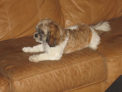
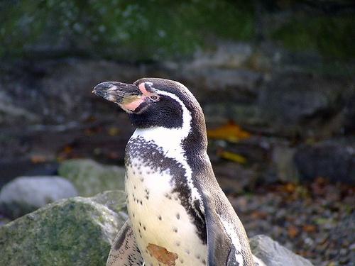
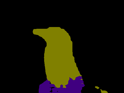
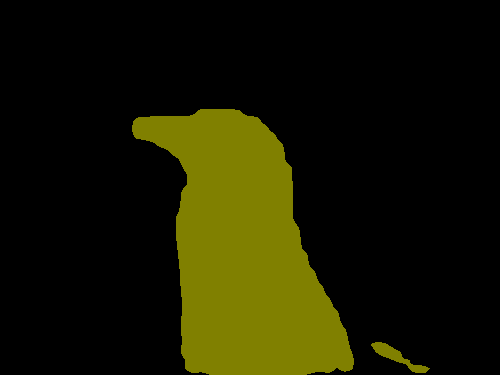

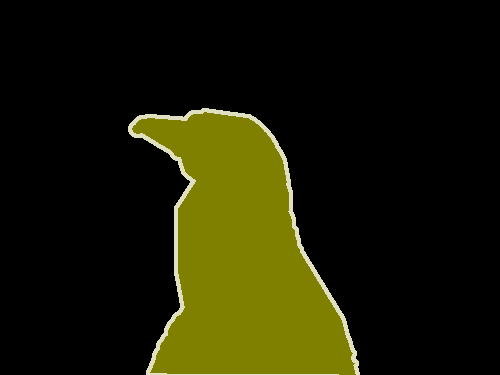








|
aero |
bike |
bird |
boat |
bottle |
bus |
car |
cat |
chair |
cow |
table |
dog |
horse |
mbike |
person |
plant |
sheep |
sofa |
train |
tv |
mean IoU | |
|---|---|---|---|---|---|---|---|---|---|---|---|---|---|---|---|---|---|---|---|---|---|
| Front end | 86.3 | 38.2 | 76.8 | 66.8 | 63.2 | 87.3 | 78.7 | 82 | 33.7 | 76.7 | 53.5 | 73.7 | 76 | 76.6 | 83 | 51.9 | 77.8 | 44 | 79.9 | 66.3 | 69.8 |
| Front + Basic | 86.4 | 37.6 | 78.5 | 66.3 | 64.1 | 89.9 | 79.9 | 84.9 | 36.1 | 79.4 | 55.8 | 77.6 | 81.6 | 79 | 83.1 | 51.2 | 81.3 | 43.7 | 82.3 | 65.7 | 71.3 |
| Front + Large | 87.3 | 39.2 | 80.3 | 65.6 | 66.4 | 90.2 | 82.6 | 85.8 | 34.8 | 81.9 | 51.7 | 79 | 84.1 | 80.9 | 83.2 | 51.2 | 83.2 | 44.7 | 83.4 | 65.6 | 72.1 |
| Front end + CRF | 89.2 | 38.8 | 80 | 69.8 | 63.2 | 88.8 | 80 | 85.2 | 33.8 | 80.6 | 55.5 | 77.1 | 80.8 | 77.3 | 84.3 | 53.1 | 80.4 | 45 | 80.7 | 67.9 | 71.6 |
| Front + Basic + CRF | 89.1 | 38.7 | 81.4 | 67.4 | 65 | 91 | 81 | 86.7 | 37.5 | 81 | 57 | 79.6 | 83.6 | 79.9 | 84.6 | 52.7 | 83.3 | 44.3 | 82.6 | 67.2 | 72.7 |
| Front + Large + CRF | 89.6 | 39.9 | 82.7 | 66.7 | 67.5 | 91.1 | 83.3 | 87.4 | 36 | 83.3 | 52.5 | 80.7 | 85.7 | 81.8 | 84.4 | 52.6 | 84.4 | 45.3 | 83.7 | 66.7 | 73.3 |
| Front end + RNN | 88.8 | 38.1 | 80.8 | 69.1 | 65.6 | 89.9 | 79.6 | 85.7 | 36.3 | 83.6 | 57.3 | 77.9 | 83.2 | 77 | 84.6 | 54.7 | 82.1 | 46.9 | 80.9 | 66.7 | 72.5 |
| Front + Basic + RNN | 89 | 38.4 | 82.3 | 67.9 | 65.2 | 91.5 | 80.4 | 87.2 | 38.4 | 82.1 | 57.7 | 79.9 | 85 | 79.6 | 84.5 | 53.5 | 84 | 45 | 82.8 | 66.2 | 73.1 |
| Front + Large + RNN | 89.3 | 39.2 | 83.6 | 67.2 | 69 | 92.1 | 83.1 | 88 | 38.4 | 84.8 | 55.3 | 81.2 | 86.7 | 81.3 | 84.3 | 53.6 | 84.4 | 45.8 | 83.8 | 67 | 73.9 |
Evaluation on the test set.
Held-out test submissions confirm the gains. Context alone beats the compared DeepLab configuration; context plus the dense conditional random field matches the cited recurrent system, and combining context with that recurrent system improves further. The original classwise table preserves the exact comparison settings and scores.
|
aero |
bike |
bird |
boat |
bottle |
bus |
car |
cat |
chair |
cow |
table |
dog |
horse |
mbike |
person |
plant |
sheep |
sofa |
train |
tv |
mean IoU | |
| DeepLab++ | 89.1 | 38.3 | 88.1 | 63.3 | 69.7 | 87.1 | 83.1 | 85 | 29.3 | 76.5 | 56.5 | 79.8 | 77.9 | 85.8 | 82.4 | 57.4 | 84.3 | 54.9 | 80.5 | 64.1 | 72.7 |
| DeepLab-MSc++ | 89.2 | 46.7 | 88.5 | 63.5 | 68.4 | 87.0 | 81.2 | 86.3 | 32.6 | 80.7 | 62.4 | 81.0 | 81.3 | 84.3 | 82.1 | 56.2 | 84.6 | 58.3 | 76.2 | 67.2 | 73.9 |
| CRF-RNN | 90.4 | 55.3 | 88.7 | 68.4 | 69.8 | 88.3 | 82.4 | 85.1 | 32.6 | 78.5 | 64.4 | 79.6 | 81.9 | 86.4 | 81.8 | 58.6 | 82.4 | 53.5 | 77.4 | 70.1 | 74.7 |
| Front end | 86.6 | 37.3 | 84.9 | 62.4 | 67.3 | 86.2 | 81.2 | 82.1 | 32.6 | 77.4 | 58.3 | 75.9 | 81 | 83.6 | 82.3 | 54.2 | 81.5 | 50.1 | 77.5 | 63 | 71.3 |
| Context | 89.1 | 39.1 | 86.8 | 62.6 | 68.9 | 88.2 | 82.6 | 87.7 | 33.8 | 81.2 | 59.2 | 81.8 | 87.2 | 83.3 | 83.6 | 53.6 | 84.9 | 53.7 | 80.5 | 62.9 | 73.5 |
| Context + CRF | 91.3 | 39.9 | 88.9 | 64.3 | 69.8 | 88.9 | 82.6 | 89.7 | 34.7 | 82.7 | 59.5 | 83 | 88.4 | 84.2 | 85 | 55.3 | 86.7 | 54.4 | 81.9 | 63.6 | 74.7 |
| Context + CRF-RNN | 91.7 | 39.6 | 87.8 | 63.1 | 71.8 | 89.7 | 82.9 | 89.8 | 37.2 | 84 | 63 | 83.3 | 89 | 83.8 | 85.1 | 56.8 | 87.6 | 56 | 80.2 | 64.7 | 75.3 |
6 Conclusion
Dilated context aggregation offers a dedicated architecture for dense prediction. Its success also shows that components inherited from classification can hurt segmentation. Failure examples remain: the method does not eliminate semantic confusion or fine-boundary errors. End-to-end dense training without classification pretraining is proposed as future work.
Acknowledgements
The authors thank Vibhav Vineet for experimental help and discussion, and Jonathan Long and the Caffe team for feedback and integration of dilated convolution.

Appendix A Urban Scene Understanding
Urban-scene experiments use the same front-end/context pattern, with context depth matched to image resolution. All reported results here omit structured prediction and train only on the training split. Front-end training uses random reflected-padding crops, SGD, and momentum; dataset-specific joint fine-tuning follows.
A.1 CamVid
CamVid uses 367 training, 100 validation, and 233 test images at 640 × 480 resolution with 11 classes. Dilation8 trains the front end for 20,000 iterations and then jointly fine-tunes front end and context. It improves on the compared systems; the original classwise results are retained.
|
Building |
Tree |
Sky |
Car |
Sign |
Road |
Pedestrian |
Fence |
Pole |
Sidewalk |
Bicyclist |
mean IoU | |
|---|---|---|---|---|---|---|---|---|---|---|---|---|
| ALE | 73.4 | 70.2 | 91.1 | 64.2 | 24.4 | 91.1 | 29.1 | 31.0 | 13.6 | 72.4 | 28.6 | 53.6 |
| SuperParsing | 70.4 | 54.8 | 83.5 | 43.3 | 25.4 | 83.4 | 11.6 | 18.3 | 5.2 | 57.4 | 8.9 | 42.0 |
| Liu and He | 66.8 | 66.6 | 90.1 | 62.9 | 21.4 | 85.8 | 28.0 | 17.8 | 8.3 | 63.5 | 8.5 | 47.2 |
| SegNet | 68.7 | 52.0 | 87.0 | 58.5 | 13.4 | 86.2 | 25.3 | 17.9 | 16.0 | 60.5 | 24.8 | 46.4 |
| DeepLab-LFOV | 81.5 | 74.6 | 89.0 | 82.2 | 42.3 | 92.2 | 48.4 | 27.2 | 14.3 | 75.4 | 50.1 | 61.6 |
| Dilation8 | 82.6 | 76.2 | 89.9 | 84.0 | 46.9 | 92.2 | 56.3 | 35.8 | 23.4 | 75.3 | 55.5 | 65.3 |
A.2 KITTI
KITTI uses 100 training and 46 test images at 1,226 × 370 resolution. The smaller vertical extent motivates removing one context layer, producing Dilation7. After front-end training, 20,000 joint-training iterations improve on the compared baselines.
|
Building |
Tree |
Sky |
Car |
Sign |
Road |
Pedestrian |
Fence |
Pole |
Sidewalk |
Bicyclist |
mean IoU | |
|---|---|---|---|---|---|---|---|---|---|---|---|---|
| Ros et al. | 71.8 | 69.5 | 84.4 | 51.2 | 4.2 | 72.4 | 1.7 | 32.4 | 2.6 | 45.3 | 3.2 | 39.9 |
| DeepLab-LFOV | 82.8 | 78.6 | 82.4 | 78.0 | 28.8 | 91.3 | 0.0 | 39.4 | 29.9 | 72.4 | 12.9 | 54.2 |
| Dilation7 | 84.6 | 81.1 | 83 | 81.4 | 41.8 | 92.9 | 4.6 | 47.1 | 35.2 | 73.1 | 26.4 | 59.2 |
A.3 Cityscapes
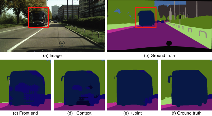
Cityscapes’ 2,048 × 1,024 images require a larger context: Dilation10 adds dilation factors 32 and 64. Training proceeds through the front end, the context module, then joint fine-tuning on image halves. The reported model improves over the contemporary compared systems; the figure and two tables preserve stagewise examples and class/category results.
|
Road |
Sidewalk |
Building |
Wall |
Fence |
Pole |
Light |
Sign |
Vegetation |
Terrain |
Sky |
Person |
Rider |
Car |
Truck |
Bus |
Train |
Motorcycle |
Bicycle |
mean IoU |
| Validation set | |||||||||||||||||||
| 97.2 | 79.5 | 90.4 | 44.9 | 52.4 | 55.1 | 56.7 | 69 | 91 | 58.7 | 92.6 | 75.7 | 50 | 92.2 | 56.2 | 72.6 | 54.3 | 46.2 | 70.1 | 68.7 |
| Test set | |||||||||||||||||||
| 97.6 | 79.2 | 89.9 | 37.3 | 47.6 | 53.2 | 58.6 | 65.2 | 91.8 | 69.4 | 93.7 | 78.9 | 55 | 93.3 | 45.5 | 53.4 | 47.7 | 52.2 | 66 | 67.1 |