At a glance
A pointer network predicts which input element to select next, so its output vocabulary grows with the input. Attention supplies a probability distribution over input positions instead of a blended context vector. Supervised experiments cover convex hulls, Delaunay triangulations, and traveling-salesman tours; generalization to larger instances is useful but uneven.
1 Introduction
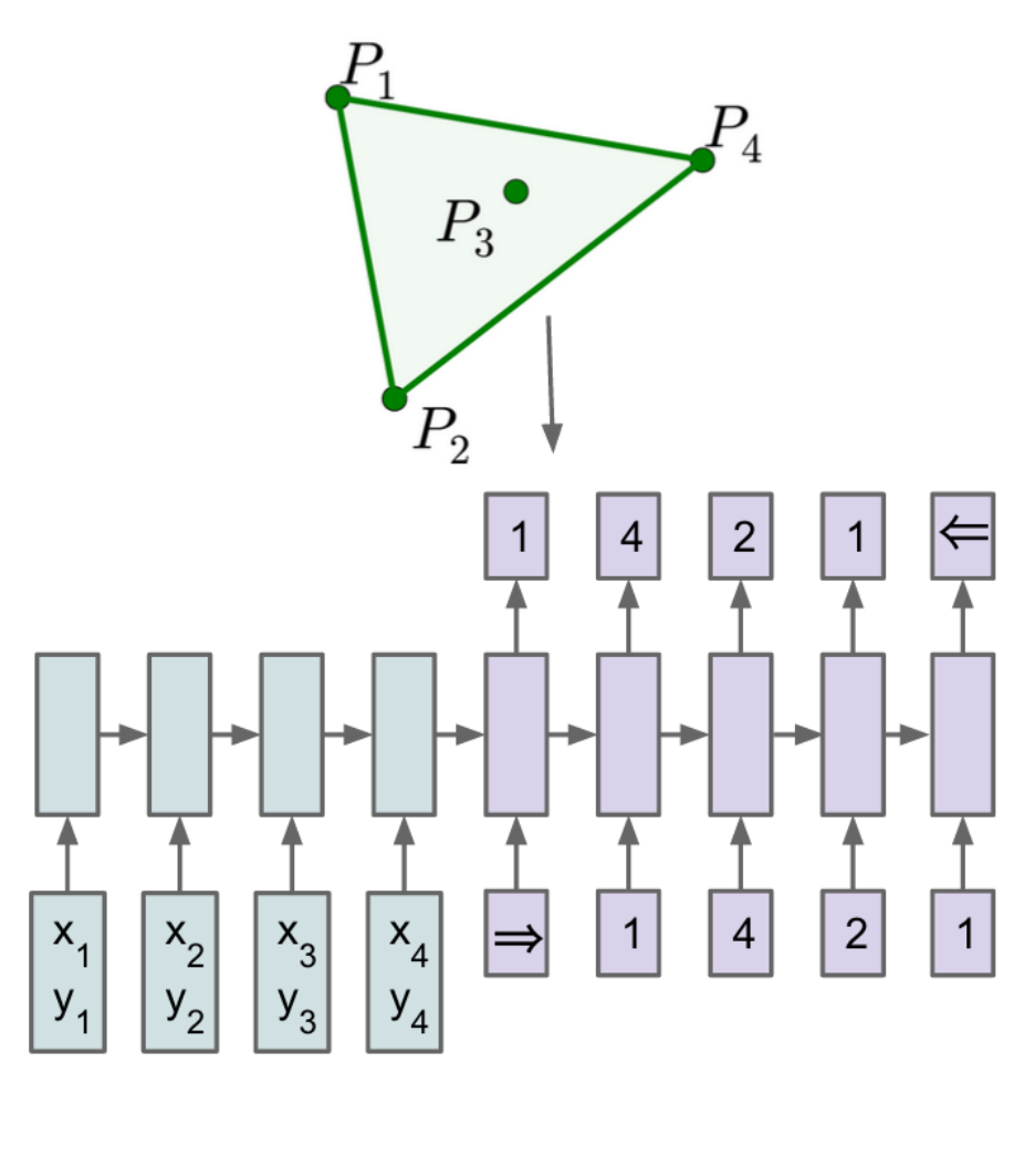
Ordinary sequence decoders predict from a fixed vocabulary, which is awkward when an answer must select members of a variable-sized input. Pointer networks reuse attention scores as the output distribution, ensuring each predicted symbol names an input position. This changes the representation of an answer without supplying an exact combinatorial solver.
2 Models
The paper develops the pointer mechanism by comparing a sequence-to-sequence baseline with an attention-augmented decoder.
2.1 Sequence-to-Sequence Model
The baseline encodes all input points and autoregressively predicts an output sequence by maximizing its conditional likelihood. A fixed output softmax cannot directly accommodate arbitrary input sizes. With output length proportional to input length, this baseline also supplies only linear decoding work, while even convex-hull algorithms generally require more computation.
Equations 1–2
| (1) |
| (2) |
2.2 Content Based Input Attention
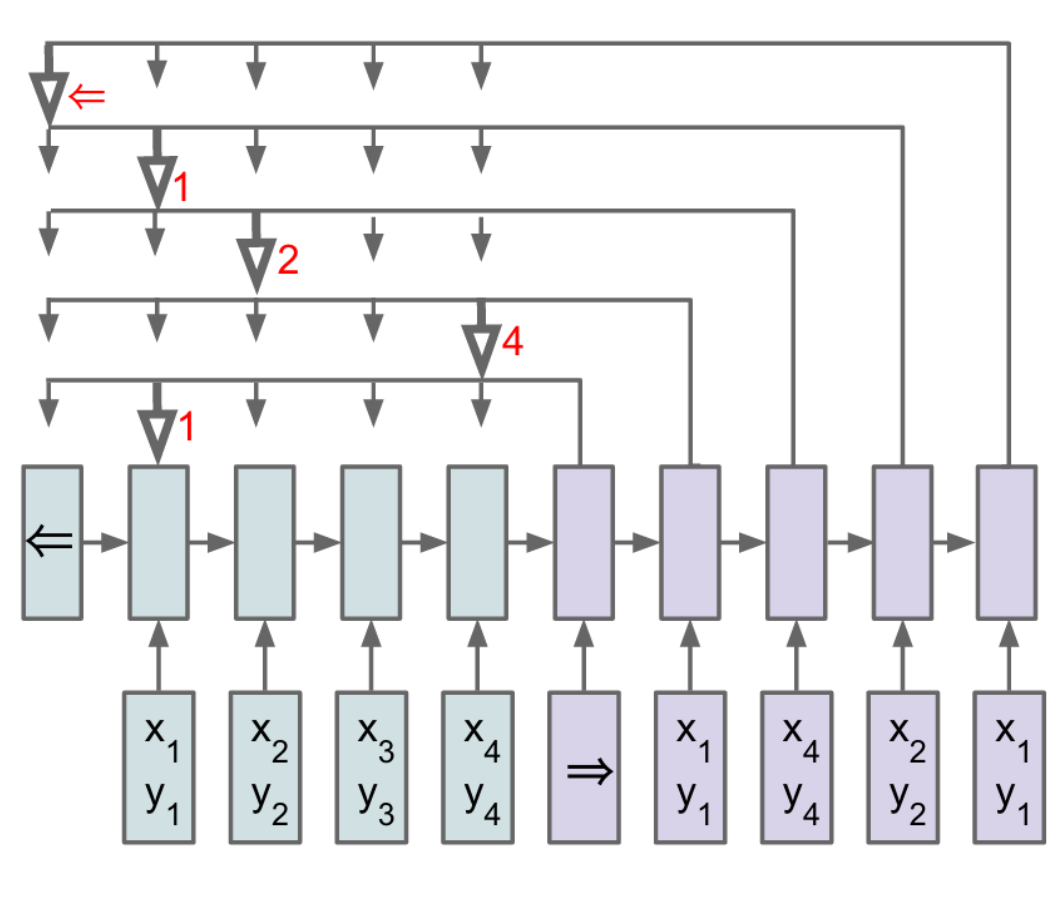
Content attention scores every encoder state against the current decoder state and forms a weighted context vector. This gives the decoder repeated access to the input and increases work to quadratic order for linear-length outputs. However, using this context with an ordinary softmax still leaves the output vocabulary fixed.
Equation 3
| (3) | |||||
2.3 Ptr-Net
The pointer decoder normalizes those attention scores directly into probabilities over input indices. After choosing an index, it feeds the corresponding input point into the next decoding step. Outputs therefore remain exact members of the input, unlike regressing approximate point coordinates. The mechanism supports different input lengths using the same learned parameters.
Equation
3 Motivation and Datasets Structure
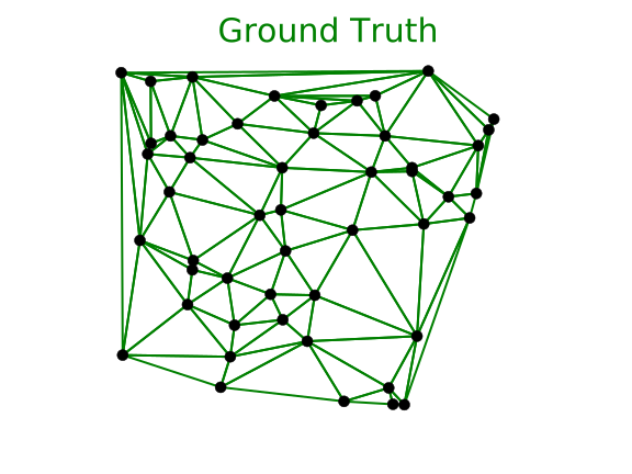
Training inputs are uniformly sampled points in the unit square. Outputs serialize geometric solutions as point indices, with chosen canonical orderings to reduce ambiguity. Figure 2 preserves the convex-hull and triangulation encodings.
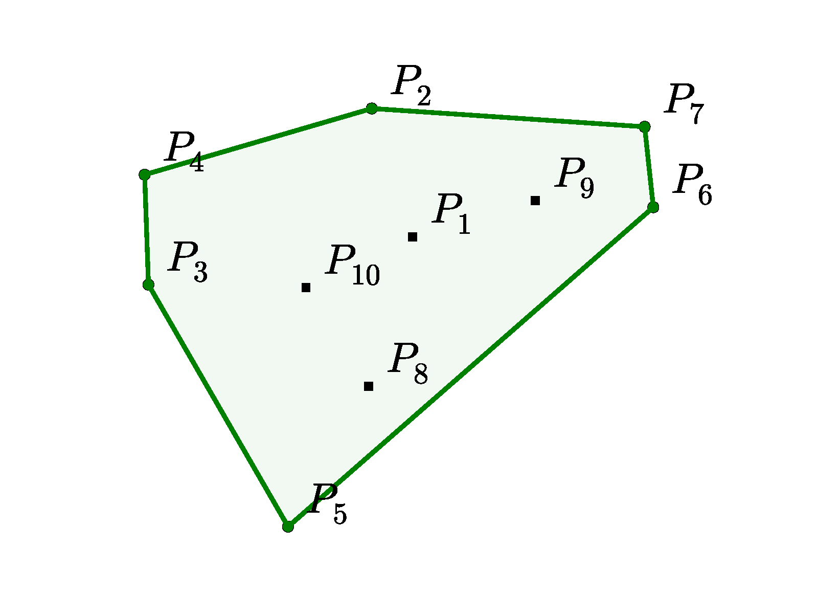
(a) Input, and the output sequence representing its convex hull.
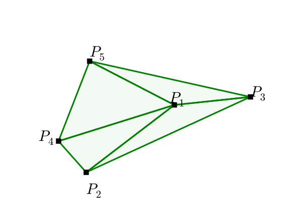
(b) Input, and the output representing its Delaunay Triangulation.
3.1 Convex Hull
A hull is represented by its boundary vertices, starting at the smallest index and proceeding counterclockwise. Exact geometric algorithms supply supervision. This deliberately fixed ordering removes equivalent cyclic descriptions and makes the learning problem easier.
3.2 Delaunay Triangulation
Each triangle is encoded as three increasing vertex indices; triangles are then sorted lexicographically by their incenters. These conventions select one sequence among many equivalent triangulations. The geometric property is that no input point lies inside any triangle’s circumcircle.
3.3 Travelling Salesman Problem (TSP)
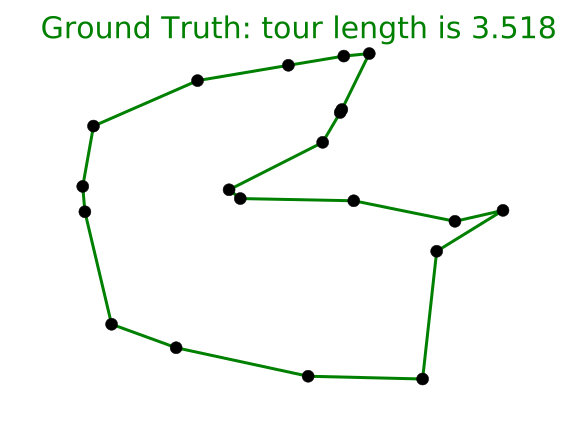
The traveling-salesman task seeks the shortest closed tour through all points. Held–Karp supplies optimal labels only for small instances, up to 20 cities; larger instances use approximate solvers. The approximation guarantees of those teachers do not transfer automatically to the learned network.
4 Empirical Results
4.1 Architecture and Hyperparameters
Models use one LSTM layer with 256 or 512 units, a million generated training pairs, minibatches of 128, gradient clipping, and a mostly shared training recipe. The authors do not conduct an extensive hyperparameter search and observe overfitting on some simpler tasks.
4.2 Convex Hull
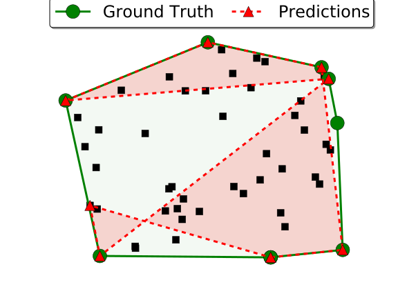
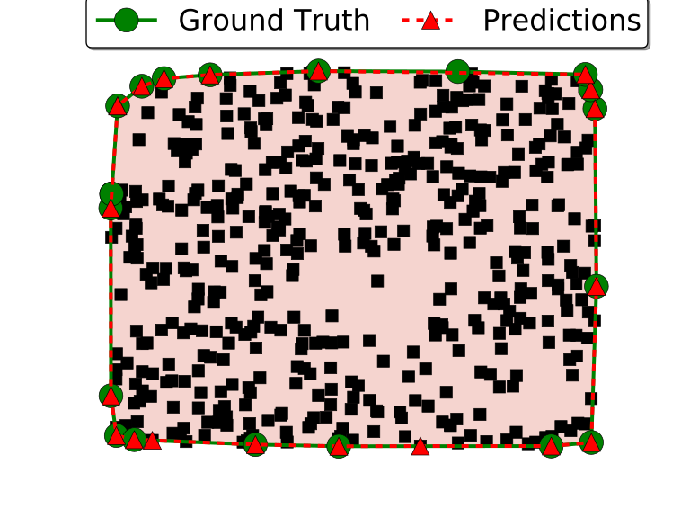
For 50-point hulls, a fixed-size pointer model reaches 72.6% exact accuracy, versus 38.9% for the attention baseline. Training on lengths 5–50 permits extrapolation to 500 points, where area coverage remains 99.2% but exact accuracy falls to 1.3%. Thus near-correct area is much easier than exact recovery. Coverage excludes invalid polygons, and settings with over 1% invalid outputs are labeled FAIL.
| Method | trained | Accuracy | Area | |
| LSTM[1] | 50 | 50 | 1.9% | FAIL |
| +attention[5] | 50 | 50 | 38.9% | 99.7% |
| Ptr-Net | 50 | 50 | 72.6% | 99.9% |
| LSTM[1] | 5 | 5 | 87.7% | 99.6% |
| Ptr-Net | 5-50 | 5 | 92.0% | 99.6% |
| LSTM[1] | 10 | 10 | 29.9% | FAIL |
| Ptr-Net | 5-50 | 10 | 87.0% | 99.8% |
| Ptr-Net | 5-50 | 50 | 69.6% | 99.9% |
| Ptr-Net | 5-50 | 100 | 50.3% | 99.9% |
| Ptr-Net | 5-50 | 200 | 22.1% | 99.9% |
| Ptr-Net | 5-50 | 500 | 1.3% | 99.2% |
4.3 Delaunay Triangulation
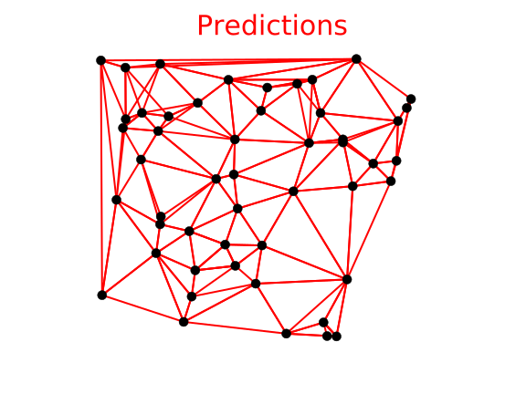
Exact triangulation accuracy drops from 80.7% at five points to 22.6% at ten, and no precisely correct triangulation is obtained at fifty. Triangle coverage remains 52.8% at fifty points. These results establish partial structure learning, not a reliable exact triangulation algorithm.
4.4 Travelling Salesman Problem
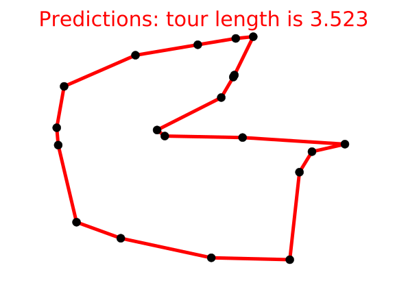
Tour decoding constrains the beam to valid tours because unconstrained outputs can repeat or omit cities. Models trained on 5–20 cities perform well at 25–30 but deteriorate markedly at 40–50. A model can sometimes surpass a weak training heuristic, yet remains an approximate learned solver with no optimality guarantee. Table 2 separates exact-label, heuristic-label, and extrapolation settings.
| Optimal | A1 | A2 | A3 | Ptr-Net | |
| 5 | 2.12 | 2.18 | 2.12 | 2.12 | 2.12 |
| 10 | 2.87 | 3.07 | 2.87 | 2.87 | 2.88 |
| 50 (A1 trained) | N/A | 6.46 | 5.84 | 5.79 | 6.42 |
| 50 (A3 trained) | N/A | 6.46 | 5.84 | 5.79 | 6.09 |
| 5 (5-20 trained) | 2.12 | 2.18 | 2.12 | 2.12 | 2.12 |
| 10 (5-20 trained) | 2.87 | 3.07 | 2.87 | 2.87 | 2.87 |
| 20 (5-20 trained) | 3.83 | 4.24 | 3.86 | 3.85 | 3.88 |
| 25 (5-20 trained) | N/A | 4.71 | 4.27 | 4.24 | 4.30 |
| 30 (5-20 trained) | N/A | 5.11 | 4.63 | 4.60 | 4.72 |
| 40 (5-20 trained) | N/A | 5.82 | 5.27 | 5.23 | 5.91 |
| 50 (5-20 trained) | N/A | 6.46 | 5.84 | 5.79 | 7.66 |
5 Conclusions
The central contribution is a variable-size output dictionary implemented through attention. The experiments show this representation can learn approximate geometric algorithms and sometimes extrapolate, while exact accuracy, output validity, and generalization differ sharply across problems.
Acknowledgments
The authors acknowledge discussions with Rafal Jozefowicz, Ilya Sutskever, Quoc Le, Samy Bengio, and manuscript help from Daniel Gillick.