Literature
Display
← All papers

Neural Turing Machines

Alex Graves · Greg Wayne · Ivo Danihelka

Preprint posted · arXiv (preprint) ↗

Contents

Overview

A Neural Turing Machine combines a neural controller with an addressable memory matrix. Differentiable reads, writes, and address shifts allow training from examples with gradient descent. Synthetic tasks show learning and some extrapolation of simple memory procedures; the system is finite and approximate, rather than an unrestricted reliable computer.

1 Introduction

An RNN may represent complex procedures in principle, yet learning them from data can be difficult. External memory provides an explicit place to store temporary variables and revisit them. The paper draws an analogy to working memory and digital computers while designing a trainable architecture rather than a biological model.

2 Foundational Research

2.1 Psychology and Neuroscience

Working-memory research motivates separating a controller from selective storage. The proposed system emphasizes flexible addressing, which is absent from many earlier neural accounts. It does not seek to reproduce human capacity limits or establish a neural implementation in the brain.

2.2 Cognitive Science and Linguistics

Variable binding and variable-length structures have long challenged connectionist models of cognition. Addressable memory offers one mechanism for assigning transient information to reusable locations. The discussion situates this design within earlier distributed representations and debates about recursive computation.

2.3 Recurrent Neural Networks

LSTM gates protect additive memory updates against vanishing or exploding sensitivity. Recurrent networks already support variable-length inputs; the new contribution is an explicitly addressable memory with learned access. Differentiable attention and earlier neural program-learning work are important precursors.

3 Neural Turing Machines

The controller receives external inputs and previous read vectors, produces outputs, and emits parameters for read and write heads. A head assigns normalized weights to memory rows rather than selecting an inherently discrete address. Sharply concentrated weights approximate ordinary memory access while retaining differentiability.
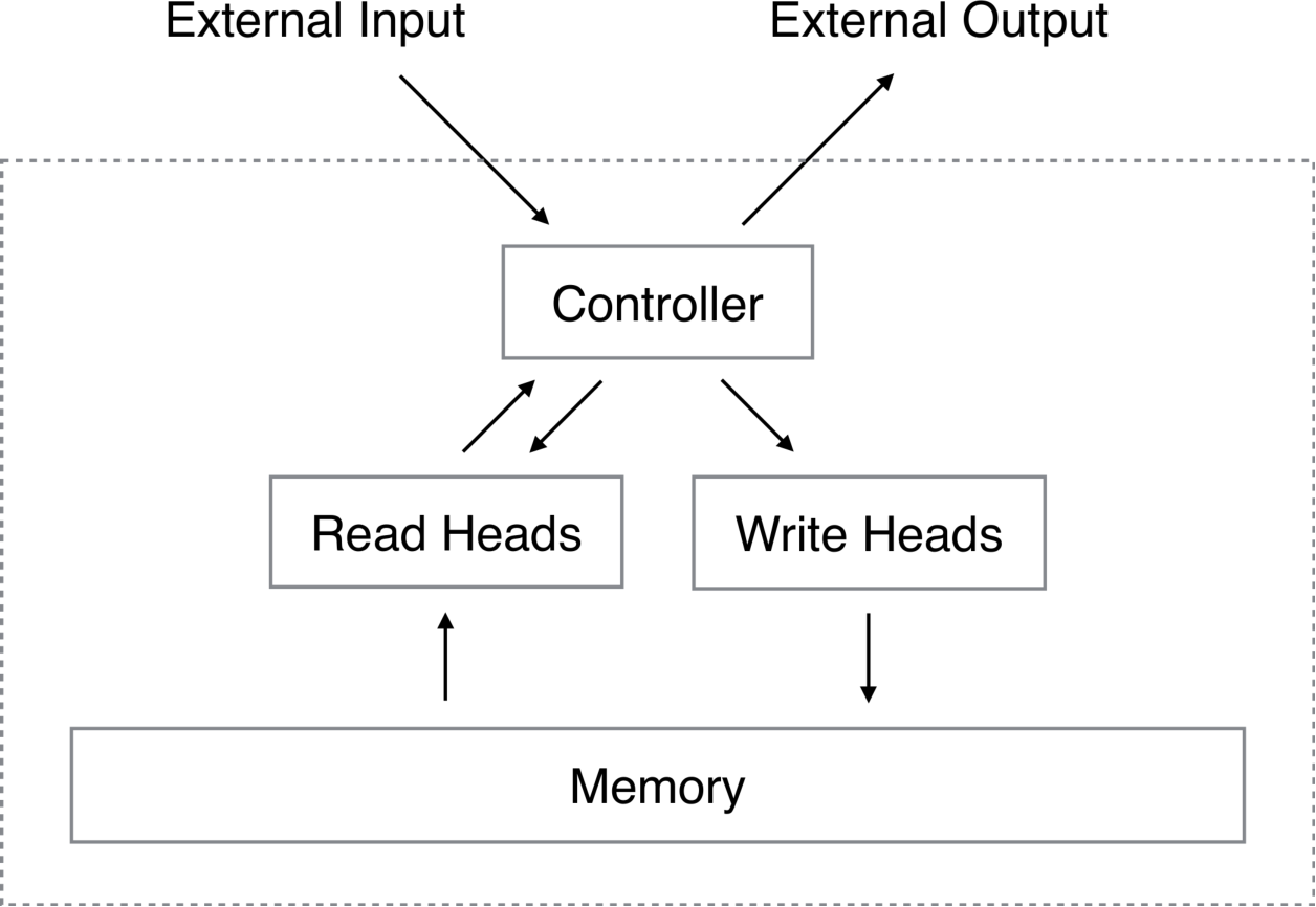
Refer to caption
Figure 1:Neural Turing Machine Architecture. During each update cycle, the controller network receives inputs from an external environment and emits outputs in response. It also reads to and writes from a memory matrix via a set of parallel read and write heads. The dashed line indicates the division between the NTM circuit and the outside world.

3.1 Reading

A read vector is the weighted average of memory rows. Its weights are nonnegative and sum to one, making the operation differentiable with respect to both memory contents and the chosen address distribution.

Equations 1–2
∑iwt(i)=1,0≤wt(i)≤1,∀i.\sum_{i}w_{t}(i)=1,\qquad 0\leq w_{t}(i)\leq 1,\,\forall i. (1)
𝐫t⟵∑iwt​(i)​𝐌t​(i),\mathbf{r}_{t}\longleftarrow\sum_{i}{w_{t}(i)\mathbf{M}_{t}(i)}, (2)

3.2 Writing

Writing first erases selected components and then adds a vector, with both operations weighted by address. Separate erase and add vectors permit fine-grained updates within a row. Multiple heads’ erase operations commute, as do their additions.

Equations 3–4
𝐌~t​(i)⟵𝐌t−1​(i)​[𝟏−wt​(i)​𝐞t],\mathbf{\tilde{M}}_{t}(i)\longleftarrow\mathbf{M}_{t-1}(i)\left[\mathbf{1}-w_{t}(i)\mathbf{e}_{t}\right], (3)
𝐌t​(i)⟵𝐌~t​(i)+wt​(i)​𝐚t.\mathbf{M}_{t}(i)\longleftarrow\mathbf{\tilde{M}}_{t}(i)+w_{t}(i)\,\mathbf{a}_{t}. (4)

3.3 Addressing Mechanisms

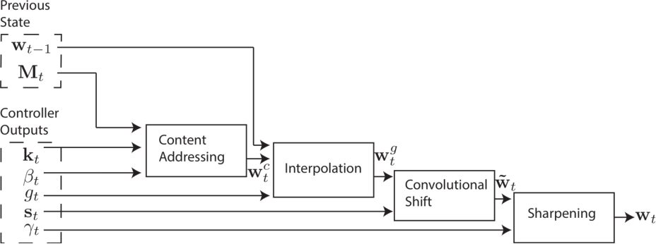
Content addressing locates a row by its stored value; location addressing moves relative to a prior position. Their combination supports both associative jumps and sequential traversal. Figure 2 shows content lookup, interpolation, shifting, and sharpening in their actual order.
Refer to caption
Figure 2:Flow Diagram of the Addressing Mechanism. Thekey vector,𝐤t\mathbf{k}_{t}, andkey strength,βt\beta_{t}, are used to perform content-based addressing of the memory matrix,𝐌t\mathbf{M}_{t}. The resulting content-based weighting is interpolated with the weighting from the previous time step based on the value of theinterpolation gate,gtg_{t}. Theshift weighting,𝐬t\mathbf{s}_{t}, determines whether and by how much the weighting is rotated. Finally, depending onγt\gamma_{t}, the weighting is sharpened and used for memory access.

3.3.1 Focusing by Content

Each head compares a learned key with all rows using cosine similarity. A positive key-strength parameter controls concentration before softmax normalization. A partial content match can therefore retrieve an associated stored vector.

Equations 5–6
wtc​(i)\displaystyle w^{c}_{t}(i) ⟵\displaystyle\longleftarrow exp⁡(βt​K​[𝐤t,𝐌t​(i)])∑jexp⁡(βt​K​[𝐤t,𝐌t​(j)]).\displaystyle\frac{\exp\bigg(\beta_{t}K\big[\mathbf{k}_{t},\mathbf{M}_{t}(i)\big]\bigg)}{\sum_{j}\exp\bigg(\beta_{t}K\big[\mathbf{k}_{t},\mathbf{M}_{t}(j)\big]\bigg)}. (5)
K⁡[𝐮,𝐯]\displaystyle K\big[\mathbf{u},\mathbf{v}\big] =\displaystyle= 𝐮⋅𝐯‖𝐮‖⋅‖𝐯‖.\displaystyle\frac{\mathbf{u}\cdot\mathbf{v}}{||\mathbf{u}||\cdot||\mathbf{v}||}. (6)

3.3.2 Focusing by Location

An interpolation gate blends the previous address distribution with a fresh content lookup. Circular convolution shifts that distribution, and an exponent then sharpens it to counter diffusion. The head can retain its position, jump by content, move relative to a match, or iterate through locations; finite circular memory can eventually wrap and overwrite data.

Equations 7–9
𝐰tg⟵gt​𝐰tc+(1−gt)​𝐰t−1.\mathbf{w}^{g}_{t}\longleftarrow g_{t}\mathbf{w}^{c}_{t}+(1-g_{t})\mathbf{w}_{t-1}. (7)
w~t​(i)\displaystyle\tilde{w}_{t}(i) ⟵∑j=0N−1wtg​(j)​st​(i−j)\displaystyle\longleftarrow\sum_{j=0}^{N-1}w^{g}_{t}(j)\,s_{t}(i-j) (8)
wt​(i)⟵w~t​(i)γt∑jw~t​(j)γtw_{t}(i)\longleftarrow\frac{\tilde{w}_{t}(i)^{\gamma_{t}}}{\sum_{j}\tilde{w}_{t}(j)^{\gamma_{t}}} (9)

3.4 Controller Network

A recurrent controller has internal state in addition to external memory, analogous to temporary registers. A feed-forward controller must use external memory for temporal information and may expose a more readable access pattern. Its number of simultaneous read heads limits how many stored vectors it can combine in one step.

4 Experiments

Five supervised synthetic tasks compare memory systems with feed-forward or LSTM controllers against a standalone LSTM. Dynamic state resets between episodes. Binary cross-entropy is reported as bits per sequence, and testing beyond training lengths probes whether a reusable procedure was learned.

4.1 Copy

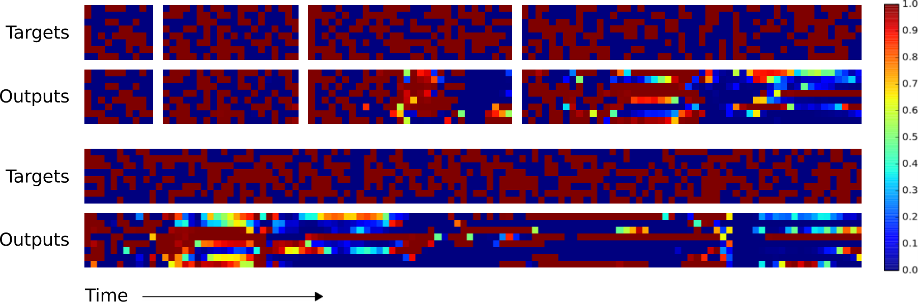
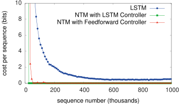
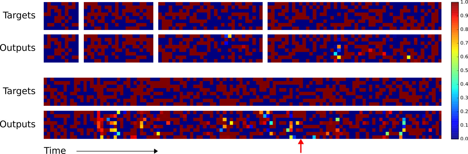
Training copies random eight-bit vectors in sequences of length 1–20. The memory models learn faster and extrapolate better than the standalone LSTM. A 120-step example still contains local mistakes and an insertion that shifts later outputs. The authors infer the preserved copy pseudocode from access traces: write sequentially, return to the start, and read sequentially. Memory capacity ultimately limits this extrapolation.
Original figure
Figure 3:Copy Learning Curves.
Refer to caption
Figure 4:NTM Generalisation on the Copy Task. The four pairs of plots in the top row depict network outputs and corresponding copy targets for test sequences of length 10, 20, 30, and 50, respectively. The plots in the bottom row are for a length 120 sequence. The network was only trained on sequences of up to length 20. The first four sequences are reproduced with high confidence and very few mistakes. The longest one has a few more local errors and one global error: at the point indicated by the red arrow at the bottom, a single vector is duplicated, pushing all subsequent vectors one step back. Despite being subjectively close to a correct copy, this leads to a high loss.
Refer to caption
Figure 5:LSTM Generalisation on the Copy Task. The plots show inputs and outputs for the same sequence lengths asFigure4. Like NTM, LSTM learns to reproduce sequences of up to length 20 almost perfectly. However it clearly fails to generalise to longer sequences. Also note that the length of the accurate prefix decreases as the sequence length increases, suggesting that the network has trouble retaining information for long periods.
initialise: move head to start location
while input delimiter not seendo
  receive input vector
  write input to head location
  increment head location by 1
endwhile
 return head to start location
while truedo
  read output vector from head location
  emit output
  increment head location by 1
endwhile
Refer to caption
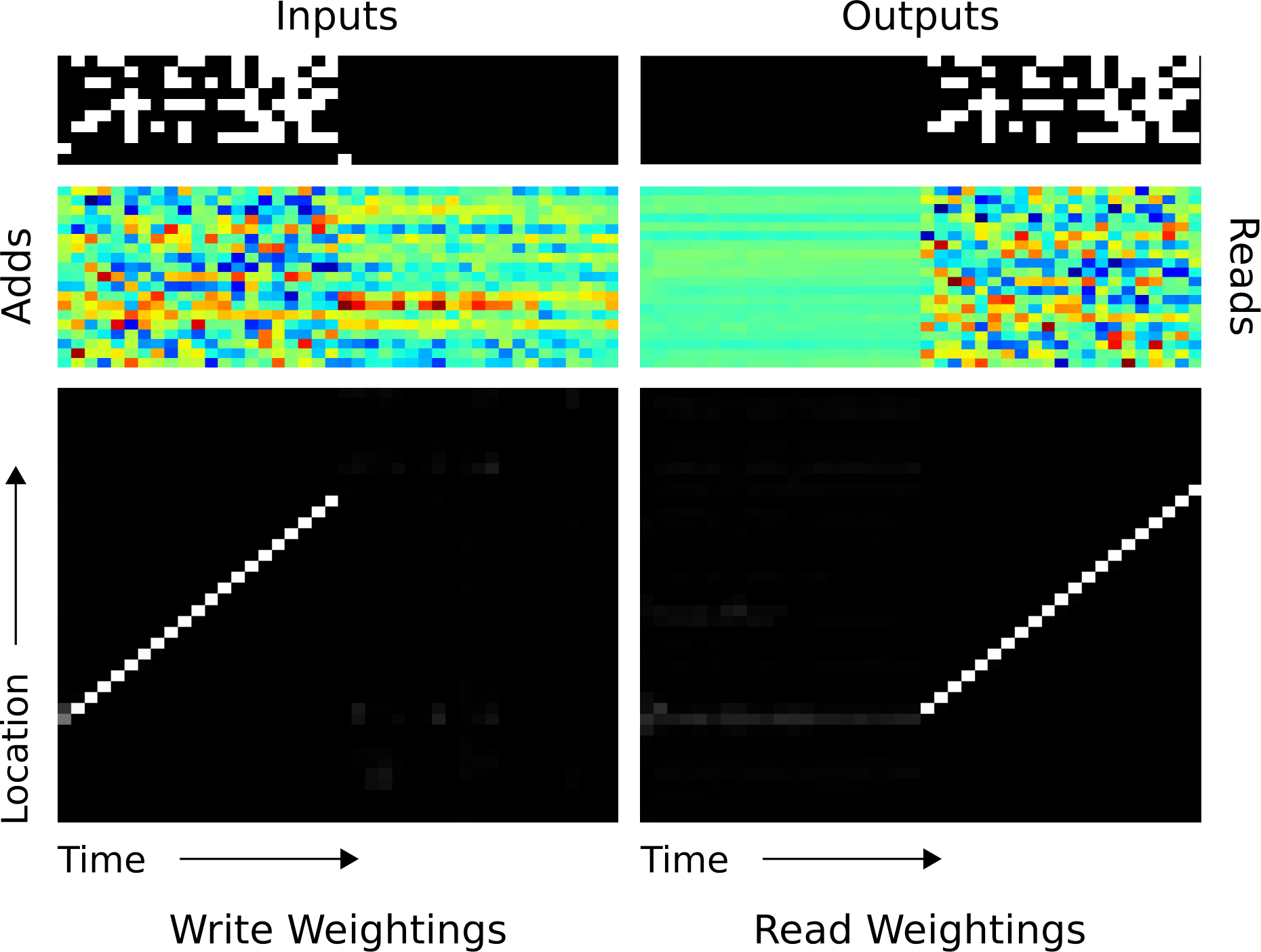
Figure 6:NTM Memory Use During the Copy Task. The plots in the left column depict the inputs to the network (top), the vectors added to memory (middle) and the corresponding write weightings (bottom) during a single test sequence for the copy task. The plots on the right show the outputs from the network (top), the vectors read from memory (middle) and the read weightings (bottom). Only a subset of memory locations are shown. Notice the sharp focus of all the weightings on a single location in memory (black is weight zero, white is weight one). Also note the translation of the focal point over time, reflects the network’s use of iterative shifts for location-based addressing, as described in3.3.2. Lastly, observe that the read locations exactly match the write locations, and the read vectors match the add vectors. This suggests that the network writes each input vector in turn to a specific memory location during the input phase, then reads from the same location sequence during the output phase.

4.2 Repeat Copy

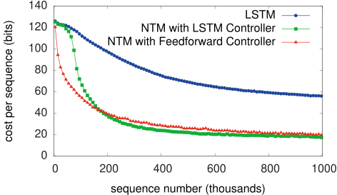
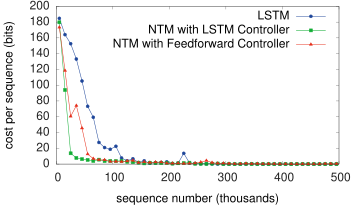
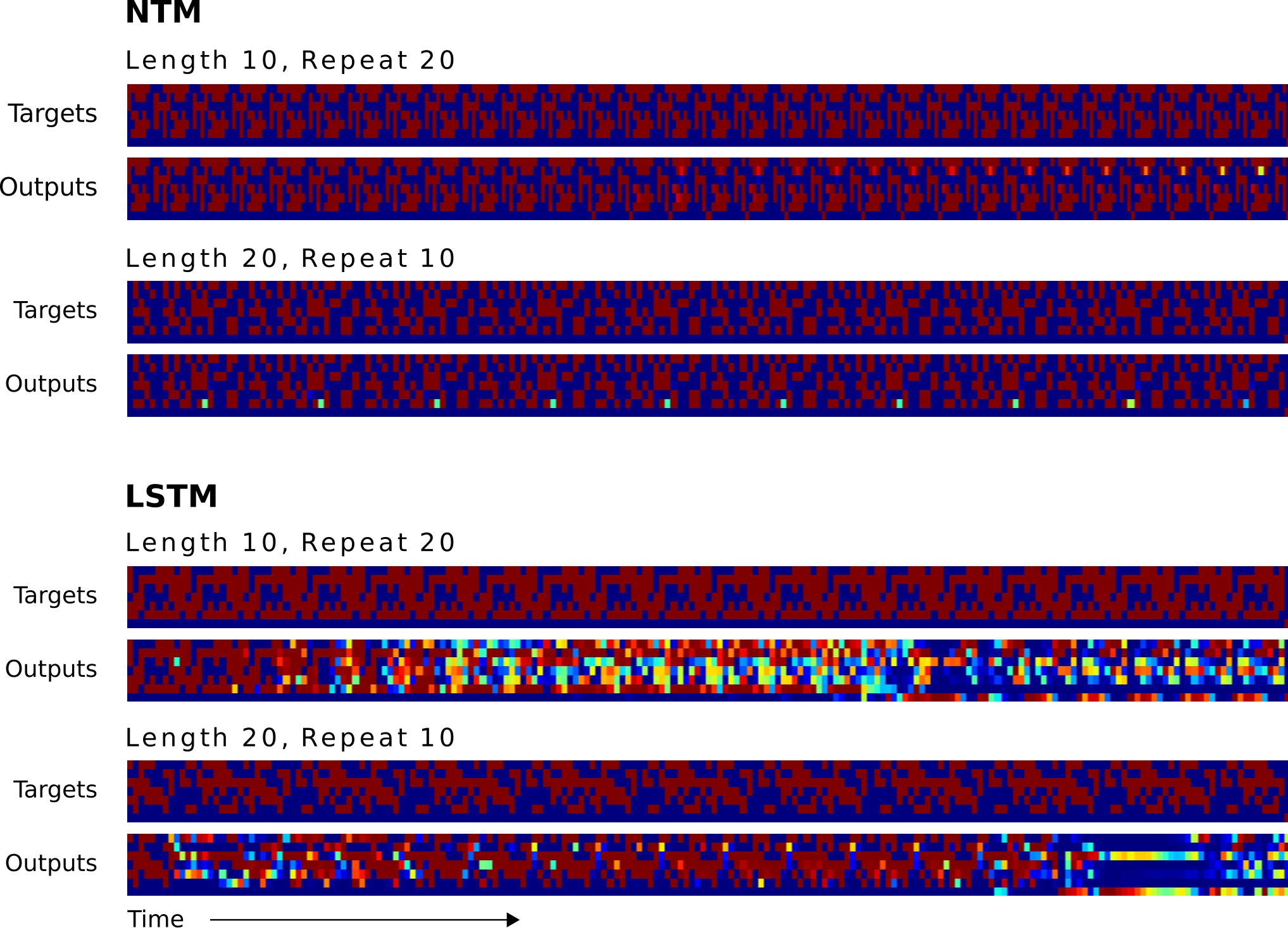
The repeat task adds a requested repetition count and an end marker. The memory model generalizes to longer input sequences, but beyond trained repetition counts it fails to stop correctly. This separates learning a reusable copying loop from learning an extrapolating numerical counter.
Original figure
Figure 7:Repeat Copy Learning Curves.
Refer to caption
Figure 8:NTM and LSTM Generalisation for the Repeat Copy Task. NTM generalises almost perfectly to longer sequences than seen during training. When the number of repeats is increased it is able to continue duplicating the input sequence fairly accurately; but it is unable to predict when the sequence will end, emitting the end marker after the end of every repetition beyond the eleventh. LSTM struggles with both increased length and number, rapidly diverging from the input sequence in both cases.
Refer to caption
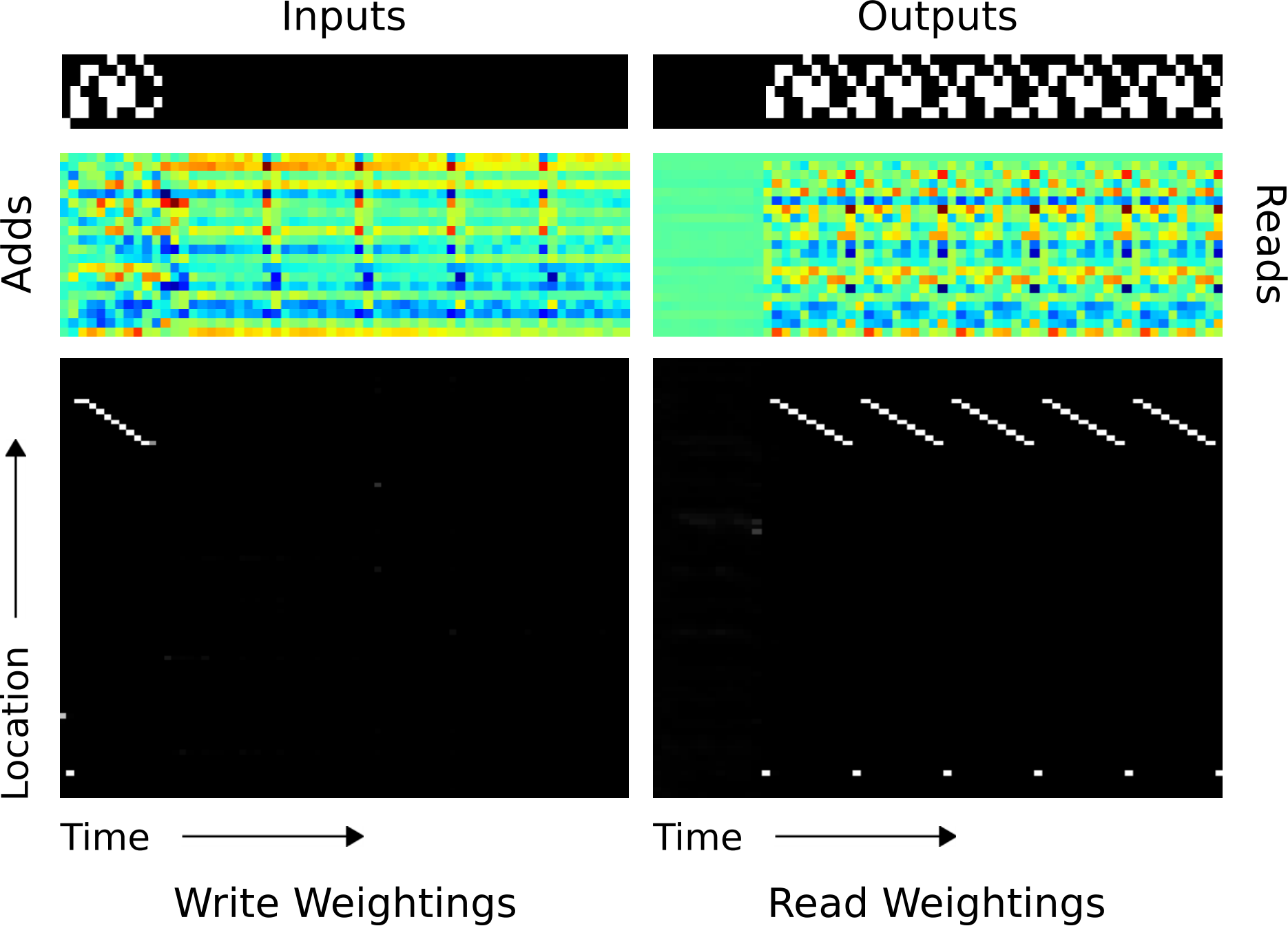
Figure 9:NTM Memory Use During the Repeat Copy Task. As with the copy task the network first writes the input vectors to memory using iterative shifts. It then reads through the sequence to replicate the input as many times as necessary (six in this case). The white dot at the bottom of the read weightings seems to correspond to an intermediate location used to redirect the head to the start of the sequence (The NTM equivalent of agoto statement).

4.3 Associative Recall

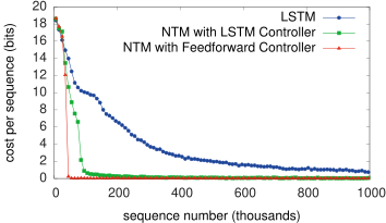
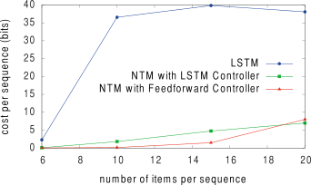
After observing several items, the network receives one as a query and must return its successor. A feed-forward controller remains nearly perfect at twice the largest training length. Traces suggest it writes a compressed key at each delimiter, retrieves that key by content, then shifts to the next item. This is the authors’ interpretation of the learned access behavior.
Original figure
Figure 10:Associative Recall Learning Curves for NTM and LSTM.
Original figure
Figure 11:Generalisation Performance on Associative Recall for Longer Item Sequences. The NTM with either a feedforward or LSTM controller generalises to much longer sequences of items than the LSTM alone. In particular, the NTM with a feedforward controller is nearly perfect for item sequences of twice the length of sequences in its training set.
Refer to caption
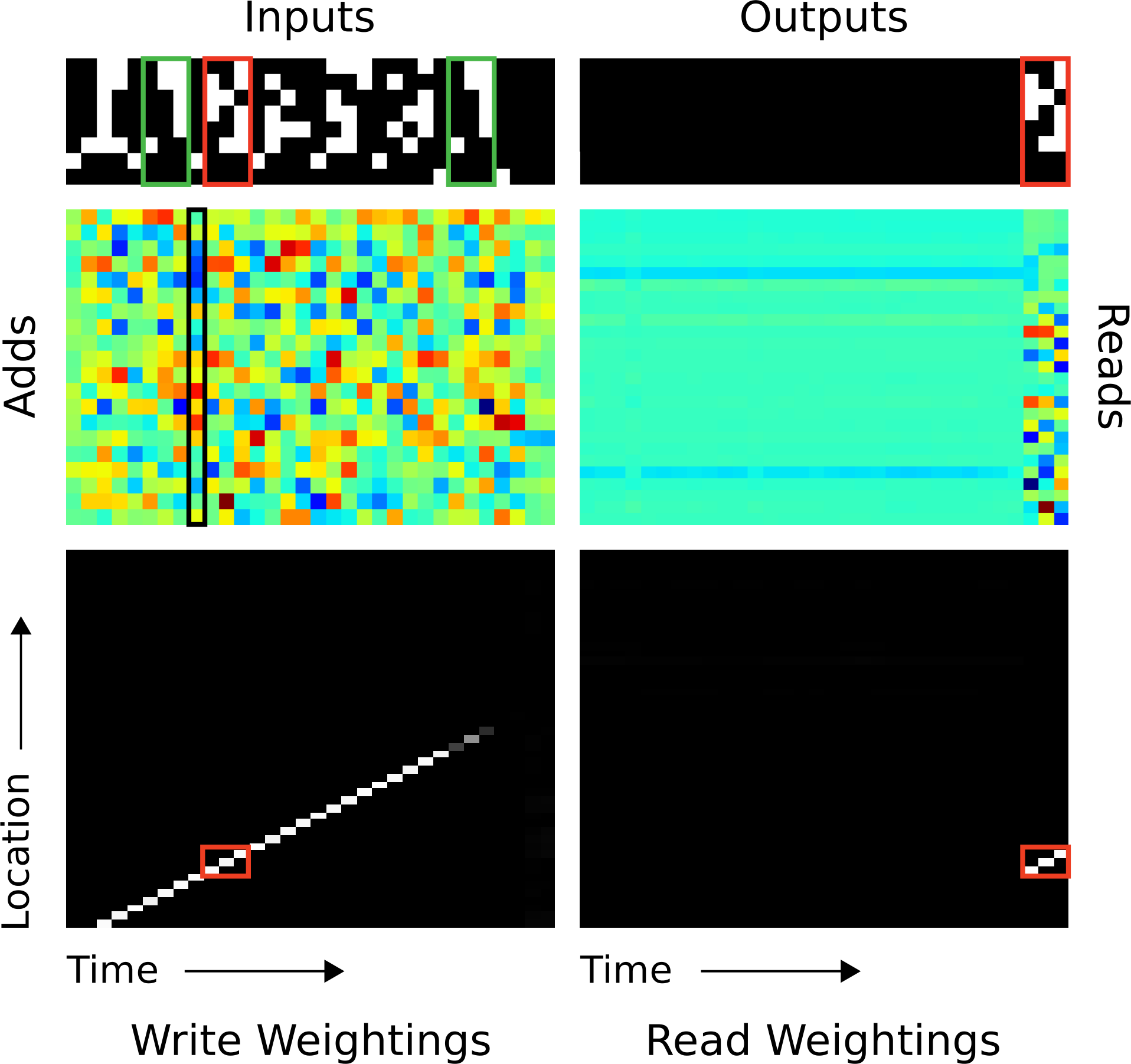
Figure 12:NTM Memory Use During the Associative Recall Task. In “Inputs,” a sequence of items, each composed of three consecutive binary random vectors is propagated to the controller. The distinction between items is designated by delimiter symbols (row 7 in “Inputs”). After several items have been presented, a delimiter that designates a query is presented (row 8 in “Inputs”). A single query item is presented (green box), and the network target corresponds to the subsequent item in the sequence (red box). In “Outputs,” we see that the network correctly produces the target item. The red boxes in the read and write weightings highlight the three locations where the target item was written and then read. The solution the network finds is to form a compressed representation (black box in “Adds”) of each item that it can store in a single location. For further analysis, see the main text.

4.4 Dynamic N-Grams

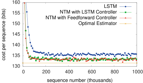
Each episode samples a new binary six-gram distribution. Predicting the next bit requires tracking the five-bit context and updating counts within the episode. The paper derives an optimal Bayesian predictor; memory models outperform the tested LSTM but do not reach it exactly. Access errors in the preserved examples expose limitations of the inferred counting mechanism.

Equation 10
P⁡(B=1|N1,N0,𝐜)=N1+12N1+N0+1P(B=1|N_{1},N_{0},\mathbf{c})=\frac{N_{1}+\frac{1}{2}}{N_{1}+N_{0}+1} (10)
Original figure
Figure 13:Dynamic N-Gram Learning Curves.
Refer to caption
Figure 14:Dynamic N-Gram Inference. The top row shows a test sequence from the N-Gram task, and the rows below show the corresponding predictive distributions emitted by the optimal estimator, NTM, and LSTM. In most places the NTM predictions are almost indistinguishable from the optimal ones. However at the points indicated by the two arrows it makes clear mistakes, one of which is explained inFigure15. LSTM follows the optimal predictions closely in some places but appears to diverge further as the sequence progresses; we speculate that this is due to LSTM “forgetting” the observations at the start of the sequence.
Refer to caption
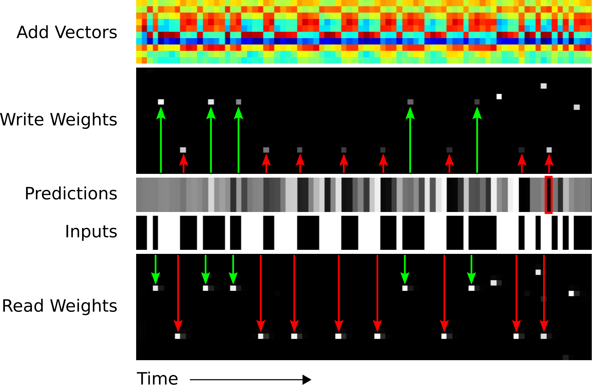
Figure 15:NTM Memory Use During the Dynamic N-Gram Task. The red and green arrows indicate point where the same context is repeatedly observed during the test sequence (“00010” for the green arrows, “01111” for the red arrows). At each such point the same location is accessed by the read head, and then, on the next time-step, accessed by the write head. We postulate that the network uses the writes to keep count of the fraction of ones and zeros following each context in the sequence so far. This is supported by the add vectors, which are clearly anti-correlated at places where the input is one or zero, suggesting a distributed “counter.” Note that the write weightings grow fainter as the same context is repeatedly seen; this may be because the memory records a ratio of ones to zeros, rather than absolute counts. The red box in the prediction sequence corresponds to the mistake at the first red arrow inFigure14; the controller appears to have accessed the wrong memory location, as the previous context was “01101” and not “01111.”

4.5 Priority Sort

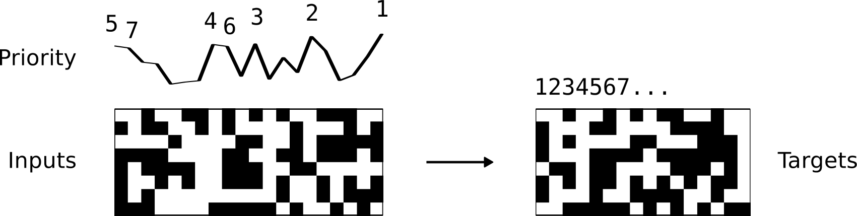
The sorting task presents twenty vectors with priorities and requests the sixteen highest-priority vectors in order. Memory access suggests writing near locations determined by priority and then reading sequentially. Both controller types outperform the LSTM baseline; the best feed-forward version uses eight read/write heads. This is a specific finite sorting task, not a proof of general exact sorting.
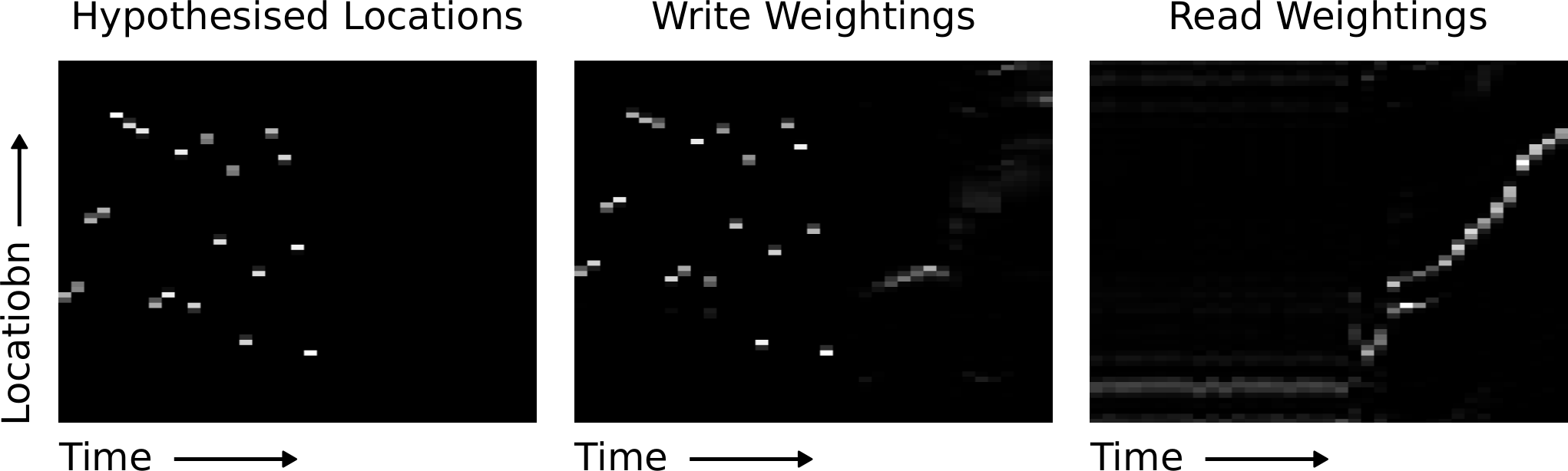
Refer to caption
Figure 16:Example Input and Target Sequence for the Priority Sort Task. The input sequence contains random binary vectors and random scalar priorities. The target sequence is a subset of the input vectors sorted by the priorities.
Refer to caption
Figure 17:NTM Memory Use During the Priority Sort Task. Left: Write locations returned by fitting a linear function of the priorities to the observed write locations. Middle: Observed write locations. Right: Read locations.
Original figure
Figure 18:Priority Sort Learning Curves.

4.6 Experimental Details

All models use RMSProp with momentum and elementwise gradient clipping. Tables 1–3 retain controller sizes, memory dimensions, learning rates, heads, and parameter counts. Adding memory rows need not add learned parameters, unlike increasing LSTM hidden width, though memory operations still cost computation.

Task #Heads Controller Size Memory Size Learning Rate #Parameters
Copy 1 100 128×\times 20 10−410^{-4} 17,16217,162
Repeat Copy 1 100 128×\times 20 10−410^{-4} 16,71216,712
Associative 4 256 128×\times 20 10−410^{-4} 146,845146,845
N-Grams 1 100 128×\times 20 3×10−53\times 10^{-5} 14,65614,656
Priority Sort 8 512 128×\times 20 3×10−53\times 10^{-5} 508,305508,305
Table 1:NTM with Feedforward Controller Experimental Settings
Task #Heads Controller Size Memory Size Learning Rate #Parameters
Copy 1 100 128×\times 20 10−410^{-4} 67,56167,561
Repeat Copy 1 100 128×\times 20 10−410^{-4} 66,11166,111
Associative 1 100 128×\times 20 10−410^{-4} 70,33070,330
N-Grams 1 100 128×\times 20 3×10−53\times 10^{-5} 61,74961,749
Priority Sort 5 2×1002\times 100 128×\times 20 3×10−53\times 10^{-5} 269,038269,038
Table 2:NTM with LSTM Controller Experimental Settings
Task Network Size Learning Rate #Parameters
Copy 3×2563\times 256 3×10−53\times 10^{-5} 1,352,9691,352,969
Repeat Copy 3×5123\times 512 3×10−53\times 10^{-5} 5,312,0075,312,007
Associative 3×2563\times 256 10−410^{-4} 1,344,5181,344,518
N-Grams 3×1283\times 128 10−410^{-4} 331,905331,905
Priority Sort 3×1283\times 128 3×10−53\times 10^{-5} 384,424384,424
Table 3:LSTM Network Experimental Settings

5 Conclusion

Differentiable external memory can make simple algorithmic tasks easier to learn and support extrapolation beyond training lengths. The demonstrations also reveal stopping, addressing, and capacity failures. The results are preliminary evidence on synthetic tasks rather than general program synthesis.

6 Acknowledgments

The authors thank colleagues from DeepMind, Google, and cognitive science for discussions and feedback.

Concept demonstration

Open image ↗