At a glance
Can a closed system become more structured while its entropy increases? The coffee automaton separates fine-grained disorder from the descriptive complexity of a smoothed state. Simulations support a rise and fall of apparent complexity for interacting particles. An apparent peak for independent particles disappears after correcting threshold artifacts; the appendix explains why their corrected complexity stays small. This is evidence about a particular model and measurement, not a proved universal law of complexity.
1 Introduction
Initially separated coffee and cream have a simple large-scale description, as does the final homogeneous mixture. Intermediate tendrils seem harder to describe. The paper asks how to measure this distinction from entropy and tests it in a stochastic cellular automaton, motivated by the broader appearance and disappearance of structure in closed systems.
2 Background
Boltzmann entropy counts microstates compatible with a chosen macrostate; Gibbs/Shannon entropy describes a probability distribution. Kolmogorov complexity measures the shortest program describing an individual string. These measures are related under suitable assumptions but all can be large for randomness, so none alone captures meaningful structure. Actual Kolmogorov complexity is uncomputable; compressed file size supplies only a computable upper bound.
Equations 1–3
| (1) |
| (2) |
| (3) |
2.1 Apparent Complexity
Apparent complexity applies an entropy or description-length measure after smoothing away incidental detail. Blurring an image can make both uniform and noisy states simple while retaining intermediate structures. The advantage is a tractable, intuitive experiment; the limitation is the chosen smoothing rule. Spatial locality motivates the rule, but does not make it unique.
2.2 Sophistication
Sophistication describes the simplest model set in which a string is a typical member, separating model structure from residual randomness. The definition uses a tolerance for incompressibility; small changes in that tolerance can substantially change the value. Coarse sophistication trades tolerance against model length instead. Both are uncomputable and harder to approximate reliably than apparent complexity. [6, 8, 10, 13]
2.3 Logical Depth
Logical depth measures the computation needed to produce a string from a near-shortest description. Random strings can be shallow because printing them is quick, whereas structured strings may require long computation. The parameter controlling near-optimality and the lack of efficient approximations complicate direct measurement. [2]
2.4 Light-Cone Complexity
Light-cone complexity uses information shared between a point’s causal past and future. It measures predictive structure in an entire space-time history rather than solely the current state. Algorithmic-information variants can be approximated with compression, but introduce different sampling and estimation problems. [12]
Equations 4–8
| (4) | ||||
| (5) |
| (6) | ||||
| (7) |
| (8) |
2.5 Synthesis
Apparent complexity can be viewed as restricting the model search in sophistication to a chosen smoothing function. Coarse sophistication is related to a Busy Beaver version of logical depth, while light-cone information may track contingent structures. These links do not make the notions interchangeable or establish an upper/lower ordering between ordinary sophistication and apparent complexity. The experiments use smoothing plus gzip because the alternatives lack an efficient estimator. [1]
Equations 9–10
| (9) |
| (10) |
3 The Coffee Automaton
A square grid begins half cream and half coffee. Two transition rules distinguish exclusion-based interactions from independent diffusion; these rules define the system being studied rather than a full fluid simulation.
3.1 Interacting Model
One particle occupies each cell. Each update chooses adjacent, different particles and swaps them. Occupancy exclusion couples their movements and can generate correlated spatial structures. This simple interaction also makes the model harder to analyze.
3.2 Non-Interacting Model
Any number of cream particles may occupy a cell; coffee is only background. At each step every cream particle takes an independent random walk. Independence makes expectations and concentration bounds tractable, providing a control against which measurement artifacts can be recognized.
4 Approximating Apparent Complexity
An implementation of OSCR produced noisy estimates and did not capture the grid’s two-dimensional structure well. The authors instead compress smoothed arrays to estimate apparent complexity and compress original arrays to estimate disorder. An attempted two-part encoding of the residual introduced its own artifacts, so these two estimates are measured separately. Generic compression remains an approximation, not an oracle for algorithmic complexity. [5, 11]
5 Coarse-Graining Experiment
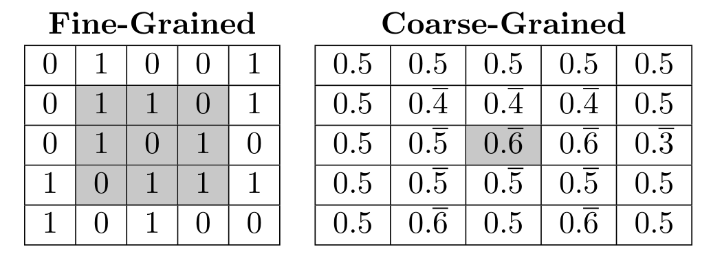
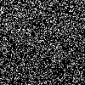
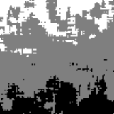
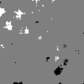
The first experiment uses a spatial moving average and a three-level threshold to distinguish coffee-rich, mixed and cream-rich regions.
5.1 Method
Average each cell’s neighborhood over a square of side g, threshold the resulting values into three levels, then measure the compressed file size. The unsmoothed array’s compressed size supplies the entropy proxy. Grain size is chosen experimentally; the measurement is therefore conditional on that resolution and encoding.
5.2 Results and Analysis
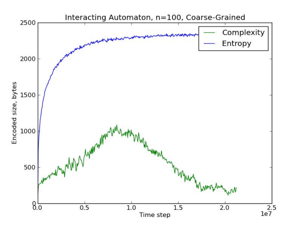
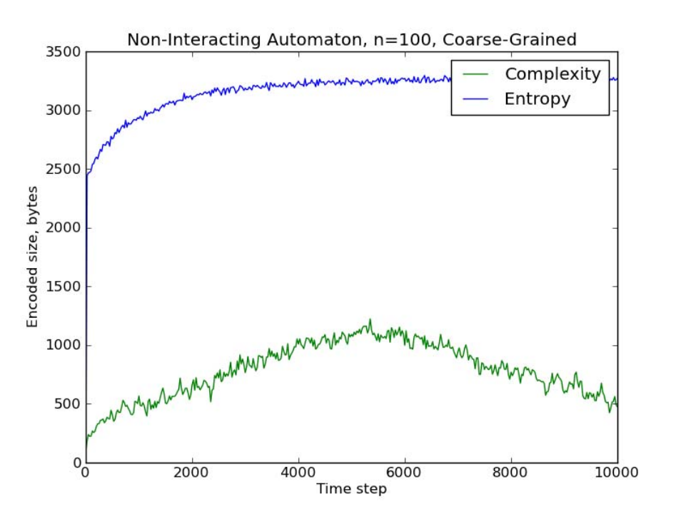
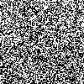
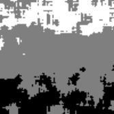
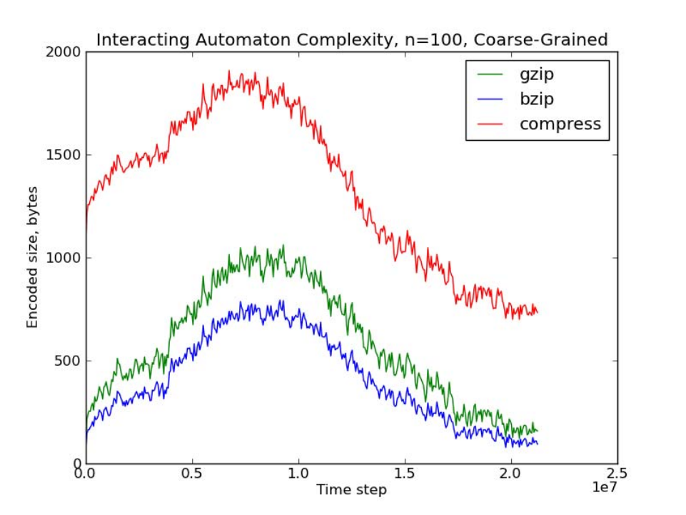
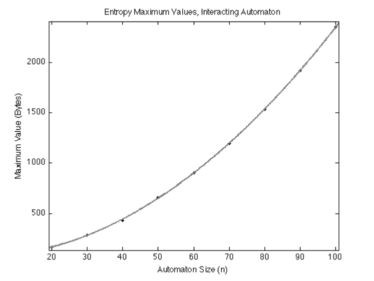
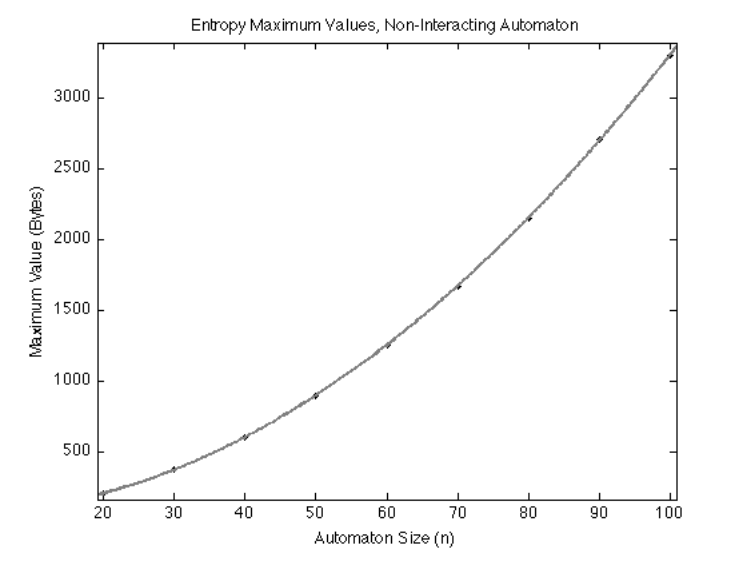
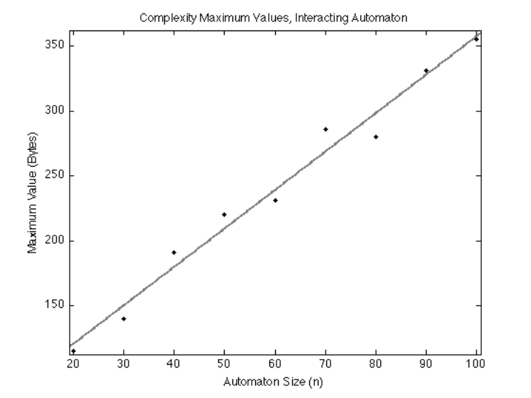
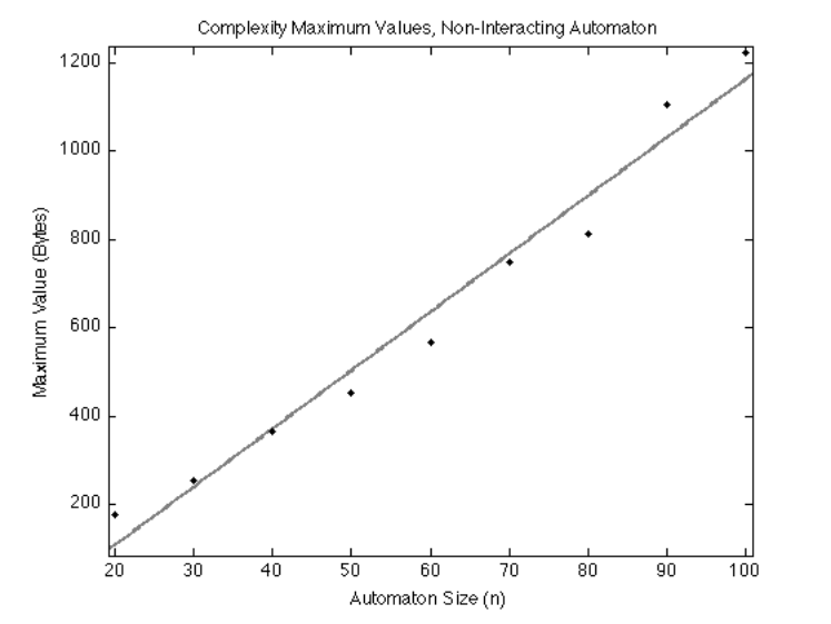
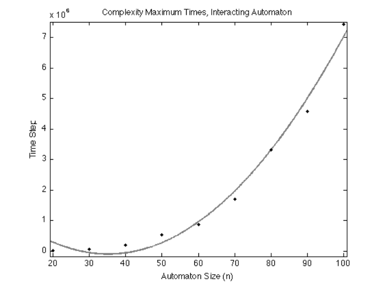
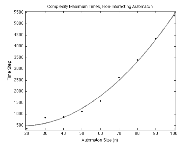
Both models initially appear to show increasing disorder and a rise then fall in apparent complexity. Across tested sizes, maximum disorder scales approximately with grid area; peak complexity scales with side length, and time to peak approximately quadratically. Alternative compressors give qualitatively similar curves. These first results are provisional: the next experiment identifies artificial complexity created by threshold crossings.
 |
 |
 |
 |
 |
 |
|
 |
 |
|
 |
 |
6 Adujsted Coarse-Graining Experiment
The revised estimator tests whether small fluctuations around threshold boundaries masquerade as meaningful spatial structure.
6.1 Method
Use seven levels and allow each pixel to shift by one level to reduce artificial boundary noise. Exact minimization would require an exponential search. The implemented approximation moves a cell to its row’s majority level when they differ by at most one. It is motivated by the initial horizontal layering and may affect structures differently in other geometries.


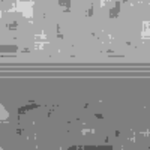
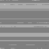
6.2 Results and Analysis
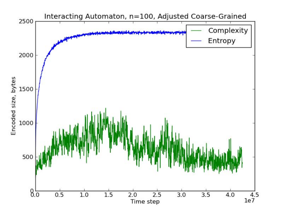
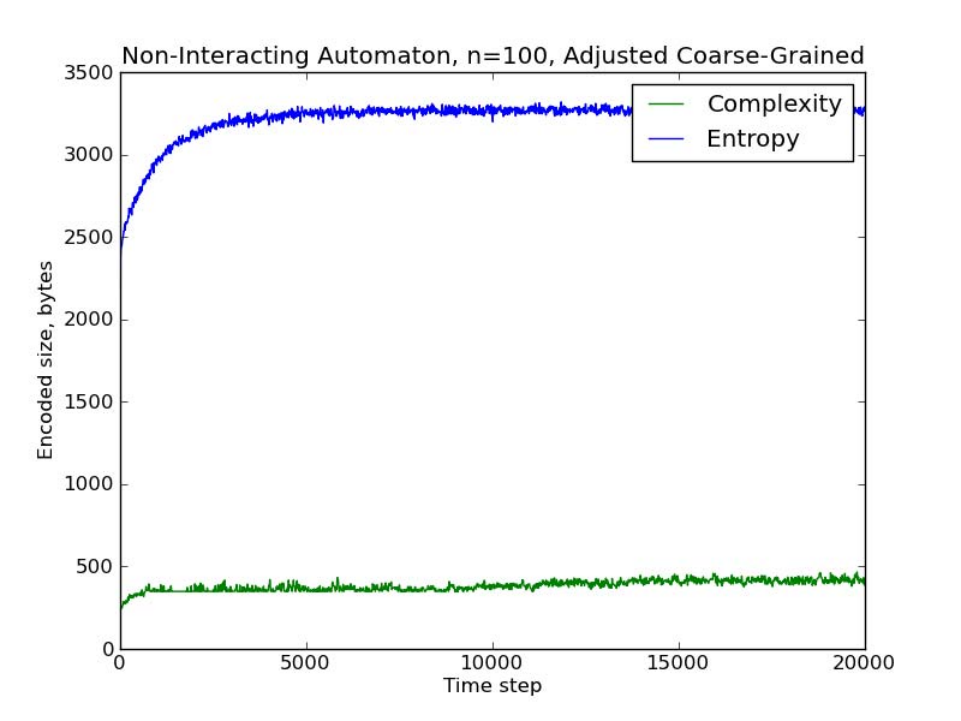
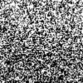
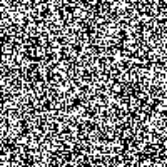
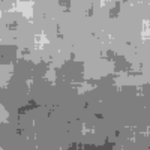
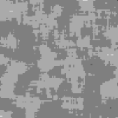
The interacting model retains a rise and fall in adjusted complexity; the independent model’s apparent peak largely disappears. Row symmetry determines the independent model’s expected density, while concentration bounds keep sufficiently large neighborhoods near that expectation. Its original peak was therefore attributable to threshold artifacts. For interacting particles the remaining peak is numerical evidence; no matching complexity lower bound is proved.
|
 |
 |
 |
 |
 |
|
 |
 |
|
 |
 |
 |
 |
 |
|
 |
 |
7 Conclusions and Further Work
Coarse-graining gives a useful but observer-dependent proxy. Alternative estimators, including light-cone information, could test robustness. A compressor establishes only an upper bound on description length, so simulations cannot prove that an intermediate state has intrinsically high algorithmic complexity. A rigorous lower bound for the interacting model remains open.
8 Acknowledgments
The authors acknowledge discussions with Alex Arkhipov, Charles Bennett, Ian Durham, Dietrich Leibfried, Aldo Pacchiano and Luca Trevisan.
9 Appendix: The Non-Interacting Case
For independent particles on a periodic grid, every cell’s expected occupancy stays at most one and depends only on its row. A Chernoff bound controls deviations of the number of particles in a square neighborhood; a union bound covers all neighborhoods at a fixed time. With grain size sufficiently larger than a constant times √log n, a one-level correction yields the row-symmetric expected pattern with high probability. Its description needs only the grid size, time and a fixed program, giving logarithmic rather than extensive complexity. The argument is a per-time high-probability bound, not a simultaneous guarantee over an unlimited history.
Equations 11–17
| (11) |
| (12) |
| (13) |
| (14) |
| (15) |
| (16) |
| (17) |