At a glance
ProMPs represent a distribution over robot trajectories rather than a single reference motion. Gaussian weights encode mean movement, time-varying variation, and correlations between joints. Conditioning adapts a movement to targets; products combine compatible behaviors; time-varying weights blend between them.
The paper derives a stochastic feedback controller under linearized dynamics and evaluates planar reaching, robot hockey, and rhythmic maracas playing. Multiple movement examples are needed to estimate useful variability; broader reinforcement-learning composition is future work.
1 Introduction
A reusable movement representation should support new targets, different speeds, coordination between joints, simultaneous behaviors, and smooth transitions. A probability distribution makes these operations explicit. Unlike a single demonstrated trajectory, it also records where motion can vary and where precision matters.
2 Probabilistic movement primitives
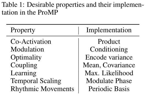
The framework unifies several desired operations through probability theory. The original property table summarizes which distribution operation supports each capability.
2.1 Trajectory representation
A trajectory is generated from basis functions and a weight vector. A Gaussian distribution over weights induces Gaussian position–velocity distributions at each time. Cross-joint weight covariance captures coordination beyond simply sharing a clock.
Equation 1

Timing and basis functions
A monotonically increasing phase variable separates movement progress from elapsed time. Changing its rate speeds up or slows down execution. Gaussian basis functions represent finite strokes; periodic von Mises bases represent rhythmic movements.
Equation 2

Joint coupling and demonstration learning
Stacking joint-specific weight vectors and basis blocks yields one distribution over the full robot motion. Maximum-likelihood or expectation-maximization fitting estimates weight mean and covariance from demonstrations. This models demonstrated variability, which is useful only to the extent the examples characterize the intended movement.
Equations 3–4


2.2 Conditioning on goals and via-points
Desired positions or velocities act as observations with a specified uncertainty. Gaussian conditioning updates the entire weight distribution, including correlations that predict compatible changes in other joints. It can condition on only part of a state, allowing coupled coordinates to adapt automatically.
Equations 5–6


Combining and blending primitives
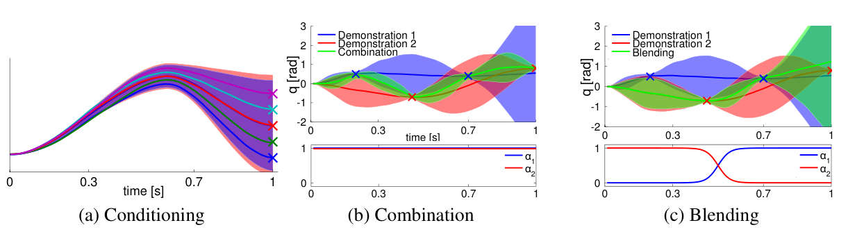
Multiplying activated primitive densities favors their overlap; smoothly varying activation weights shifts the movement between primitives. Gaussian products have summed precision and a precision-weighted mean. Figure 1 illustrates conditioning, simultaneous via-point constraints, and a transition between two movements.
The original equations are preserved as printed. In Eq. 8, the mean expression prints an inverse on the combined covariance; the standard Gaussian-product mean instead multiplies the weighted precision sum by the combined covariance.
Equations 7–8


2.3 From a distribution to feedback control
The model-based controller linearizes local dynamics and uses time-varying linear feedback, feed-forward action, and Gaussian control noise. Matching the next-state mean and covariance to the desired distribution yields moment constraints. These claims rely on the stated linear-Gaussian model and realizability assumptions, rather than guaranteeing arbitrary nonlinear trajectory distributions.
Equations 9–13





Controller gains
Taking the small-time-step limit converts covariance matching into a differential equation. Solving it with a pseudoinverse of the control matrix gives the feedback gain. The desired covariance must be invertible where the formula uses its inverse, and the requested dynamics must be realizable by the available controls.
Equations 14–17




Feed-forward control
After choosing feedback gains, matching the desired mean derivative determines the feed-forward term. Inverse-dynamics control can simplify the system matrices to a constant linear model.
Equations 18–19


Control-noise estimation
The desired joint distribution of consecutive states supplies cross-time covariance. Matching it to the forward model determines system-noise covariance, which is converted to control-noise covariance through the control-matrix pseudoinverse. This computation precedes gain estimation.
Equations 20–22



3 Experiments
Evaluation includes a simulated seven-link arm and two tasks on a physical seven-joint KUKA lightweight arm. These are demonstrations of distribution reproduction, conditioning, and composition, rather than a large task-success benchmark.
Seven-link reaching
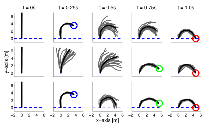
Demonstrations from an optimal controller reach a final target at one second and an intermediate target at either 0.25 or 0.75 seconds. [22] Separate ProMPs reproduce those behaviors; their product reaches both intermediate constraints. Joint variation remains large where allowed while end-effector variation is small at via-points.
Robot hockey
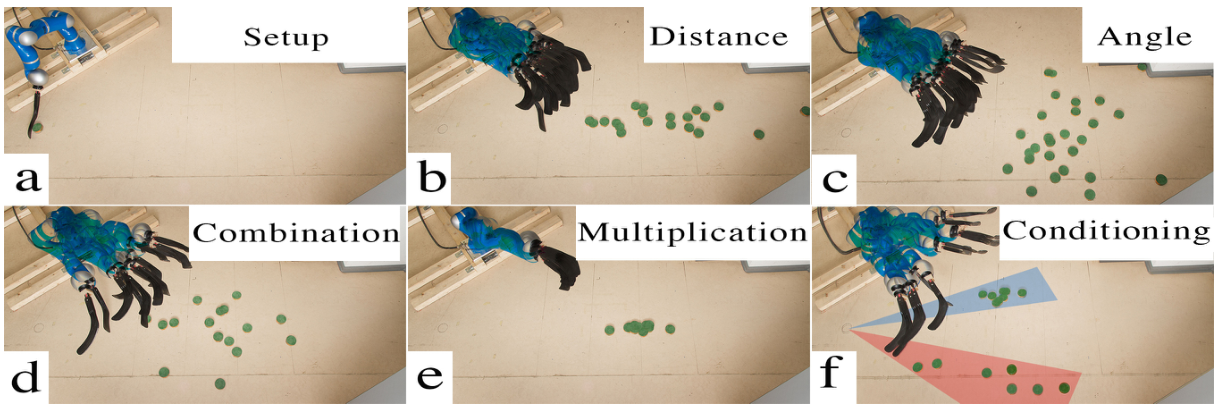
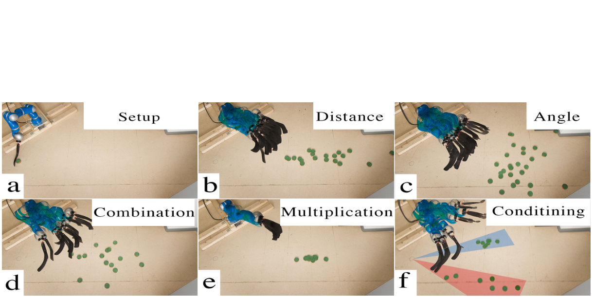
Ten demonstrations vary straight-shot distance and ten vary shooting angle. Separately learned models reproduce those forms of variation. Training on their union permits both; multiplying the models instead selects their overlap—roughly straight, medium-distance shots. Conditioning jointly modeled movement weights and final puck angle selects a desired direction.
Rhythmic maracas playing
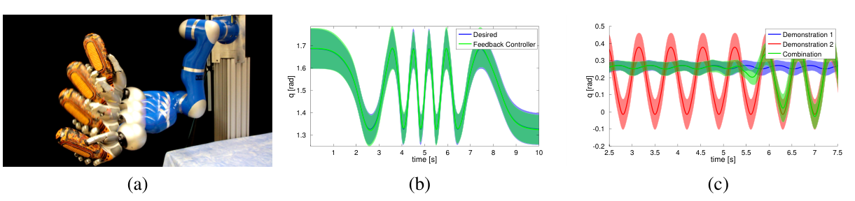
A slow demonstration of about ten periods teaches a rhythmic motion that is later accelerated by changing phase speed. A second sideways rhythm supports smooth transitions between patterns. The robot hand holds the instrument; the learned primitives control the arm.
4 Conclusion
The Gaussian trajectory representation supports modulation, blending, coupling, and a model-based feedback realization in one framework. Reinforcement-learning improvement and a broader modular control architecture remain proposed extensions. Funding supported the reported research.
Supplement: reaching protocol and comparison
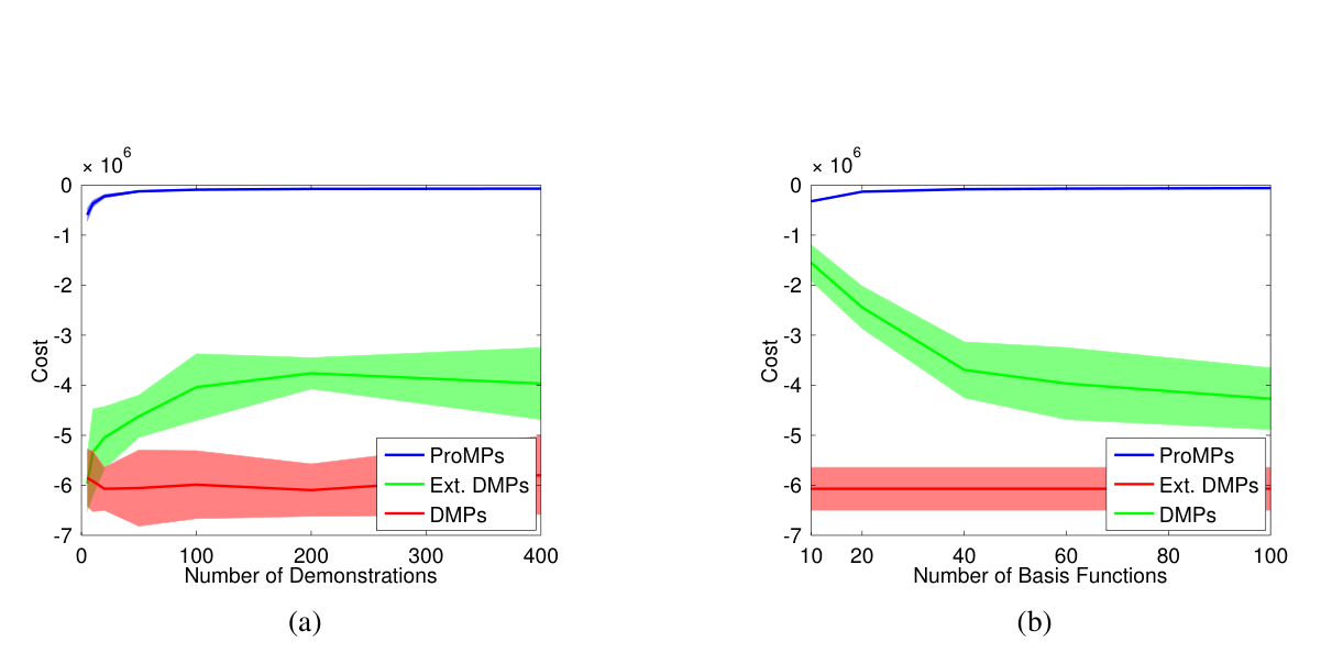
Two sets of twenty planner-generated demonstrations use control-noise covariance 200I. Sixty bases per joint produce 420 weights and a 420×420 covariance. The supplement compares ProMPs, conventional DMPs, and a variable-gain DMP modification over 200 reproductions per setting. ProMPs better match timed via-points and achieve costs comparable to the demonstration controller; the comparison varies both demonstrations and basis count.
Supplement: physical hockey implementation
The KUKA arm uses its Fast Research Interface with a one-millisecond control step. ProMP accelerations are integrated to desired positions. Kinesthetic demonstrations train ten Gaussian bases per joint, totaling seventy weights. Product composition requires no new demonstrations; direction conditioning fits a joint distribution over weights and final puck angle.
Supplement: rhythmic learning
The seven-joint arm carries a fifteen-joint DLR hand that only holds the instrument. A slow ten-period demonstration is divided into 400 parts with phase labels, and ten von Mises bases per joint are fitted using expectation maximization. Changing phase speed and blending a second demonstrated rhythm produce different sound patterns.