At a glance
Intuition. Imagine tuning two control knobs: one barely changes the output, while the other changes it sharply. Equal knob movements are therefore not equal changes to the model. Natural gradient measures the change in predicted probabilities and adjusts the step accordingly, including interactions between knobs.
Reading the math. In F⁻¹g, g is the usual loss gradient and F measures local statistical sensitivity. If F is diagonal with entries 4 and 1 and g=(1,1), the adjusted direction is (¼,1): the more sensitive coordinate moves less. The learning rate sets the overall step size; singular F requires additional treatment.
A parameter step should be measured in the geometry of the model. Amari derives the natural gradient as the inverse metric times the ordinary gradient, studies its online statistical efficiency, and works out metrics for perceptrons, invertible matrices and linear systems. This is an analytic paper; it does not benchmark contemporary language models.
Its main optimality claim is asymptotic and conditional: under a regular realizable likelihood model and convergence to the true parameter, a particular online rule matches the leading covariance of optimal batch maximum likelihood. Plateau avoidance is a separate motivation supported here by cited preliminary studies.
1 · Introduction
Ordinary gradients depend on the chosen coordinates. Equal Euclidean parameter steps can represent unequal changes in the model. A Riemannian metric makes the local notion of step length explicit and changes which direction is steepest.
The introduction distinguishes online estimation, which uses each arriving example once, from batch estimation, which can revisit observations. It also motivates an adaptive learning rate for tracking changing targets. Statistical efficiency, optimization speed and tracking performance are different questions.
2 · Natural gradient and Theorem 1
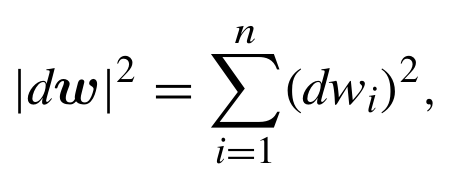
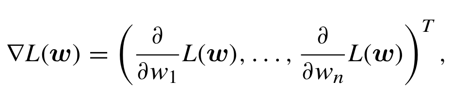
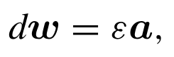
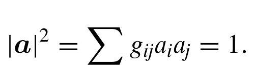
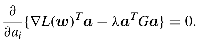
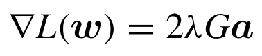
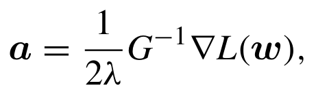
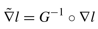
The squared local length of a displacement is its quadratic form under a positive-definite metric tensor. Linearizing the loss and minimizing its first-order change at fixed metric length gives a direction proportional to minus the inverse metric times the gradient. The proof uses a Lagrange multiplier to fix normalization.
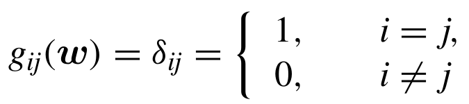
In orthonormal Euclidean coordinates the metric is the identity, so the natural and ordinary gradients agree. This is a local infinitesimal statement with an invertible metric. Finite discrete steps still need a suitable learning rate; singular statistical models need further treatment.
Equations PDF p.2 · display 1–PDF p.4 · display 15







3 · Natural-gradient learning
Independent observations with a common distribution define an expected loss. A stochastic update uses the current observation and a positive-definite preconditioning matrix. Natural-gradient learning chooses that matrix to be the inverse metric.
The expected risk defines the target, while the observation-level loss supplies a noisy update. A geometric choice of metric does not imply that each realized stochastic loss decreases at every iteration.


3.1 · Statistical density estimation
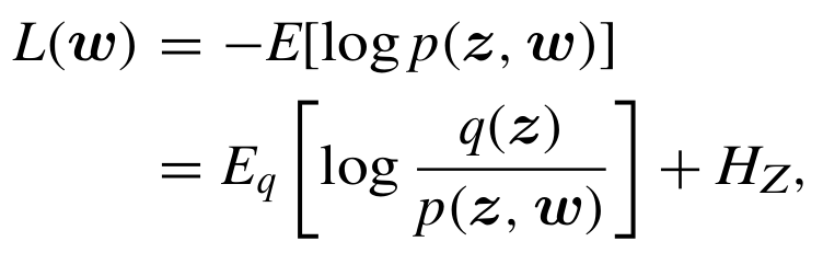
Negative log likelihood has expected value equal to KL divergence from the data distribution to the model plus a parameter-independent entropy term. The statistical model carries a Fisher metric formed from expected outer products of log-density derivatives.
This measures local changes in probability distributions instead of raw coordinate distances. The full metric includes correlations between directions. A practical diagonal second-moment optimizer is not automatically the exact Fisher inverse used here.



3.2 · Multilayer networks as statistical models
Gaussian output noise turns squared prediction error into negative log likelihood up to parameter-independent terms, giving a feedforward network a probabilistic model and Fisher metric. The construction depends on the output-noise model and input law.
Source-reading note: the printed second factor in Eq 3.11 omits log, unlike the score-product definition in Eq 3.5 and the later explicit calculation. Its original display is preserved; the reading interpretation uses the Fisher definition rather than this apparent typographic inconsistency.






3.3 · Blind separation of sources
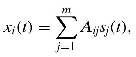
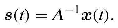
Independent source signals pass through an unknown nonsingular mixing matrix; an adaptive demixing matrix seeks to recover them. A zero expected update at the desired solution is necessary but does not establish stability. The paper distinguishes general transformations of an estimating function from a positive-definite metric applied to a loss gradient.
The model also includes unknown source-density functions and is therefore semiparametric. Omitting those nuisance functions would incorrectly turn the problem into an ordinary fully specified likelihood model. The printed product in Eq 3.12 repeats the first density subscript; the intended independence factorization is over the respective source densities.
Equations PDF p.7 · display 28–PDF p.8 · display 39










3.4 · Blind source deconvolution
Convolutive mixing includes delayed source signals. The demixing model is a matrix-valued finite impulse response filter whose coefficients use present and past observations. Defining its natural gradient requires geometry on a space of systems.
The section sets up notation for Section 8. Eq 3.23 prints the same delay exponent for every coefficient despite describing a degree-d filter; the original is retained, while the interpretation follows the coefficient-dependent filter expansion used elsewhere.







4 · Fisher-efficient online learning
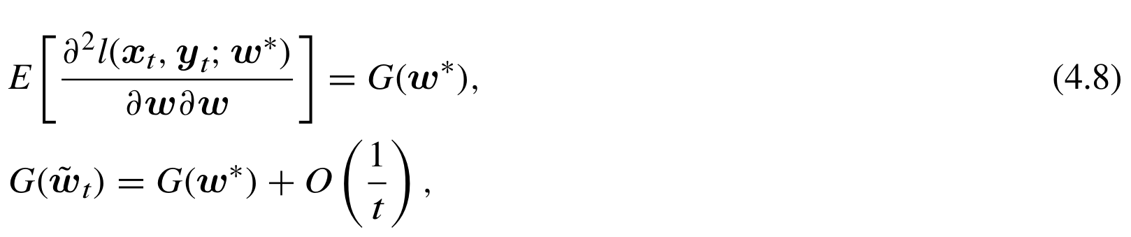
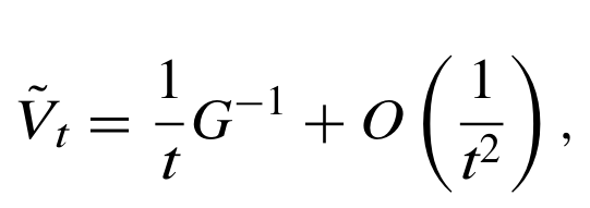
For a realizable teacher, independent examples, a regular likelihood model, and convergence to the true parameter, Theorem 2 gives leading estimation-error covariance equal to inverse Fisher information divided by t when the natural-gradient learning rate is 1/t. This matches the asymptotic covariance of optimal batch maximum likelihood.
The proof expands the stochastic gradient near the true parameter and uses the zero expected score and equality between expected likelihood curvature and Fisher information. A covariance recurrence yields the leading term. The stochastic-approximation conditions invoked in the proof matter; this is not global convergence from an arbitrary starting point.
Equations PDF p.10 · display 47–PDF p.12 · display 59










4 · Misspecification and semiparametric exceptions
For an unrealizable teacher, the paper replaces Fisher information with the appropriate expected loss Hessian to recover the corresponding optimal-batch asymptotic result. It relates that local procedure to Newton–Raphson learning, distinguishing it from the realizable Fisher identity.
For blind source separation and deconvolution, unknown source densities can invalidate the theorem and stability of the true solution. The paper explicitly withholds its efficiency theorem unless the true densities are correctly estimated and used. These are limitations of the result itself.
Equation PDF p.12 · display 60

5 · Adaptive learning constant
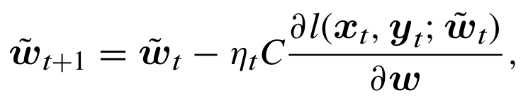
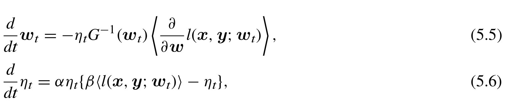
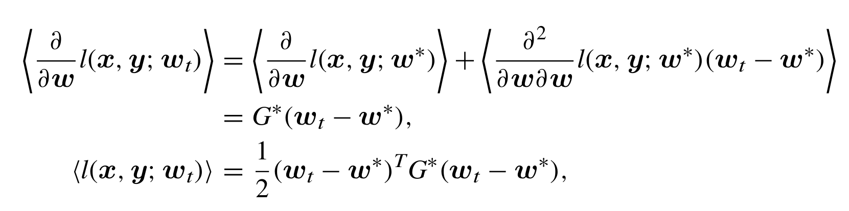
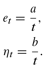
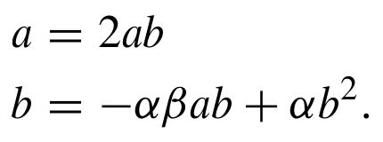
The proposed coupled rule updates parameters by natural gradient and changes the learning rate multiplicatively using the current loss and the learning rate itself. Its analysis assumes a realizable deterministic teacher with zero optimal expected loss, passes to continuous time and averages over incoming examples.
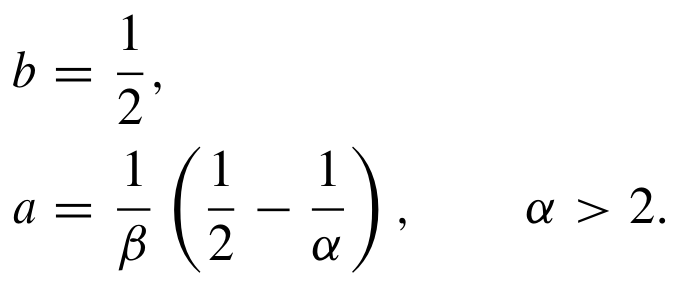
Near the optimum, a metric-weighted quadratic error and the learning rate obey a two-variable differential system. A 1/t-form solution has explicit coefficients under the displayed parameter condition. This supports the analyzed local averaged decay rate, rather than a general guarantee for every changing target or stochastic network.
Equations PDF p.13 · display 61–PDF p.14 · display 71






6 · Explicit perceptron geometry: Theorems 3–4
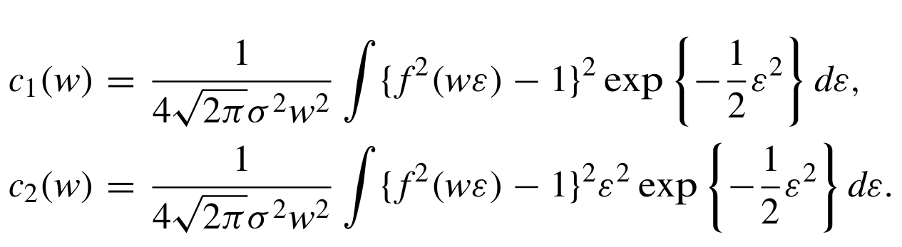
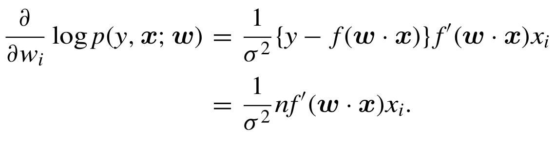
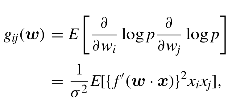
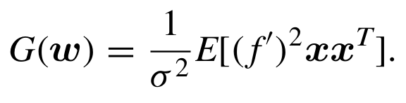
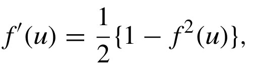
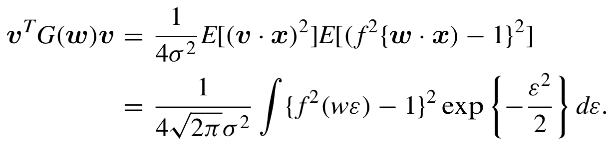
For a single sigmoidal perceptron with isotropic Gaussian inputs and Gaussian output noise, symmetry reduces Fisher information to an identity term and a rank-one term along the weight vector. Two one-dimensional Gaussian integrals determine the coefficients.
The proof evaluates quadratic forms parallel and perpendicular to the weights. The same eigenspace decomposition gives a closed-form inverse and natural-gradient update without general dense inversion. This formula depends on the specified model and input law.
Equations PDF p.14 · display 72–PDF p.17 · display 89












6 · Volume, invariant prior and multilayer blocks
The metric determinant induces a volume element and an invariant prior. The paper gives formulas and states finite model volume for this perceptron family. Eq 6.10 includes a normalization inconsistent with identifying its left side as the unnormalized volume density; the preceding Eq 6.9 distinguishes the normalized prior. Both displays are retained as printed.
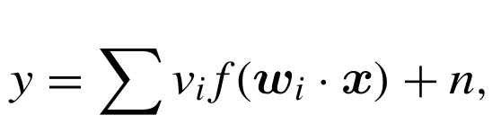
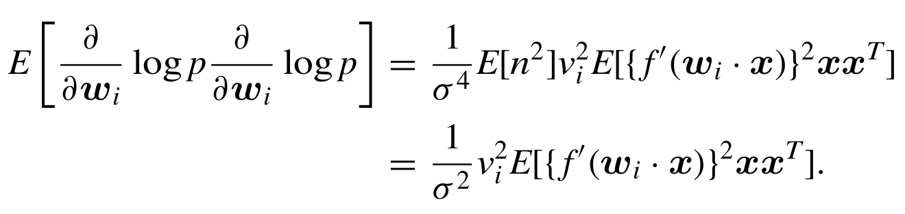
For a multilayer perceptron, diagonal and cross-unit Fisher blocks contain correlated activation derivatives. Rotational structure reduces the studied inversion problem, but inversion remains nontrivial. The cited preliminary plateau observations do not prove that all multilayer plateaus disappear.







7 · Geometry of invertible matrices: Theorem 6
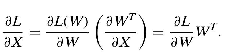
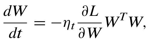
Invertible square matrices form a Lie group. A right-invariant metric transports a displacement at W to the identity by right multiplication with W inverse and measures it with the Frobenius inner product. The resulting natural gradient right-multiplies the ordinary gradient by W-transpose times W.
The derivation uses a local nonholonomic frame: these transported differentials need not integrate into a single global coordinate function. This chosen invariant matrix geometry should not be equated automatically with an arbitrary probability model’s full Fisher tensor.
Equations PDF p.19 · display 99–PDF p.20 · display 109









7 · Demixing updates and stability
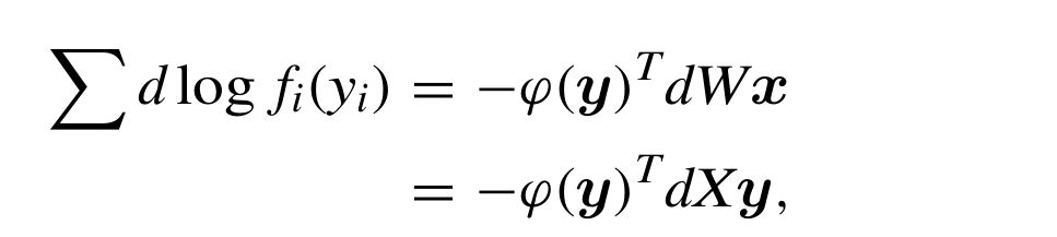
The demixing objective combines a log determinant with log source-density models. Differentiating in the transported frame gives an identity term and an output/score outer-product correction, followed by multiplication by W. As printed, Eq 7.11 uses a transposed-score product inconsistent with the stated column-vector convention; the source is preserved, not silently made executable.
The Hessian in this frame decomposes into diagonal entries and small coupled blocks under the cited analysis, facilitating stability checks. Correct density modeling still matters for efficiency and stability; Lie-group geometry does not remove those statistical requirements.







8 · Systems-space natural gradient: Theorem 7
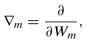
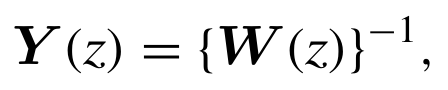
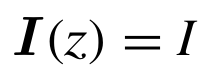
The construction repeats the invariance principle for matrix filters. A displacement is transported to the identity system, where the metric sums squared coefficient entries. The theorem gives a natural direction using the ordinary gradient and time-reversed transposed filter factors.
The proof is omitted in the source. The resulting direction need not be causal or finite impulse response, so additional delay and mapping steps are needed for a causal finite-order online method. The paper states the geometric principle and explicitly defers those implementation details.
Equations PDF p.22 · display 118–PDF p.23 · display 130









9 · Conclusions
Three levels of argument should remain separate: local metric steepest descent, conditional asymptotic efficiency for online likelihood estimation, and explicit geometry in tractable model spaces. Each has its own assumptions and computational costs.
This edition condenses explanatory prose while preserving the mathematical displays and all references. The original has no scientific figures or data tables. Claims of statistical optimality retain Section 4’s regularity and semiparametric exceptions; plateau avoidance remains a suggestion supported by the studies cited in the paper.