At a glance
SPACE reconstructs speech from millimeter-wave radar measurements of a loudspeaker’s vibration. A speaker-conditioned Radio TransUNet first predicts a speech Mel spectrogram; a neural vocoder then generates its waveform. A frequency transformation layer helps infer missing high-frequency structure, while a speaker encoder supports variation across voices.
Experiments replay TIMIT recordings from 630 speakers through a loudspeaker. SPACE improves objective speech metrics and listener naturalness ratings over the tested reconstruction baselines, including on 63 held-out voices. The evidence concerns supervised, stationary loudspeaker playback under specified laboratory conditions, rather than direct recovery of arbitrary live human conversations.
I. Introduction
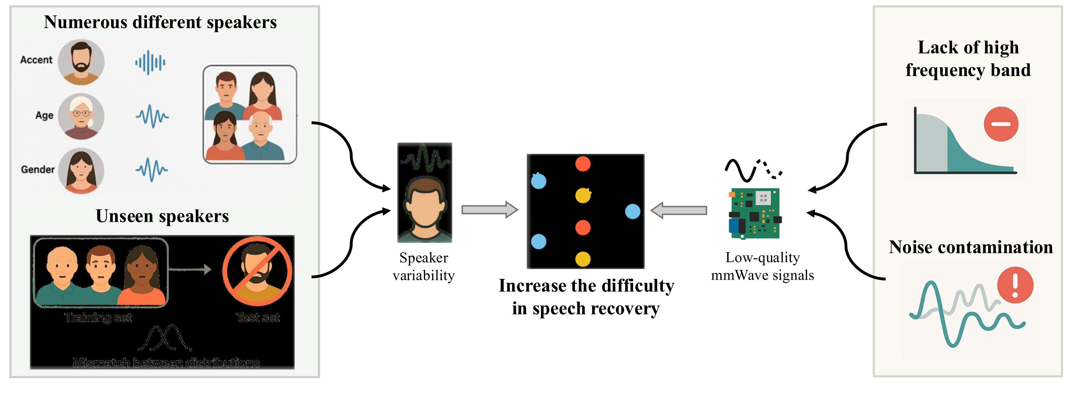
Radio sensing can reveal speech-related mechanical vibration even when an ordinary microphone is affected by acoustic noise or some barriers. Existing systems face two linked problems: voices vary, and radar observations lack much of the clean speech spectrum and contain phase noise. Figure 1 illustrates these challenges.
SPACE addresses them through explicit speaker conditioning, frequency mixing, and vocoder-based synthesis. Prior work already explored unseen speakers; the claimed advance is improved recovery with a larger speaker population and low-quality inputs, not the first demonstration of any speaker generalization.
II. Preliminary knowledge
The sensing background explains why phase variations can carry vibration information and why the resulting signal is only a partial observation of speech.
A. Vibration sensing
A vibrating object changes the round-trip delay of a reflected frequency-modulated continuous-wave signal. Equation 1 preserves the intermediate-frequency signal model. The method identifies the target reflection, removes static clutter, and follows unwrapped phase variation across chirps to estimate vibration.
The phase is more sensitive to tiny motion than directly resolving the corresponding frequency change. This physical relation motivates recovery, but does not imply that every speech frequency or phoneme is directly measured.
Equation

B. Feasibility and challenges
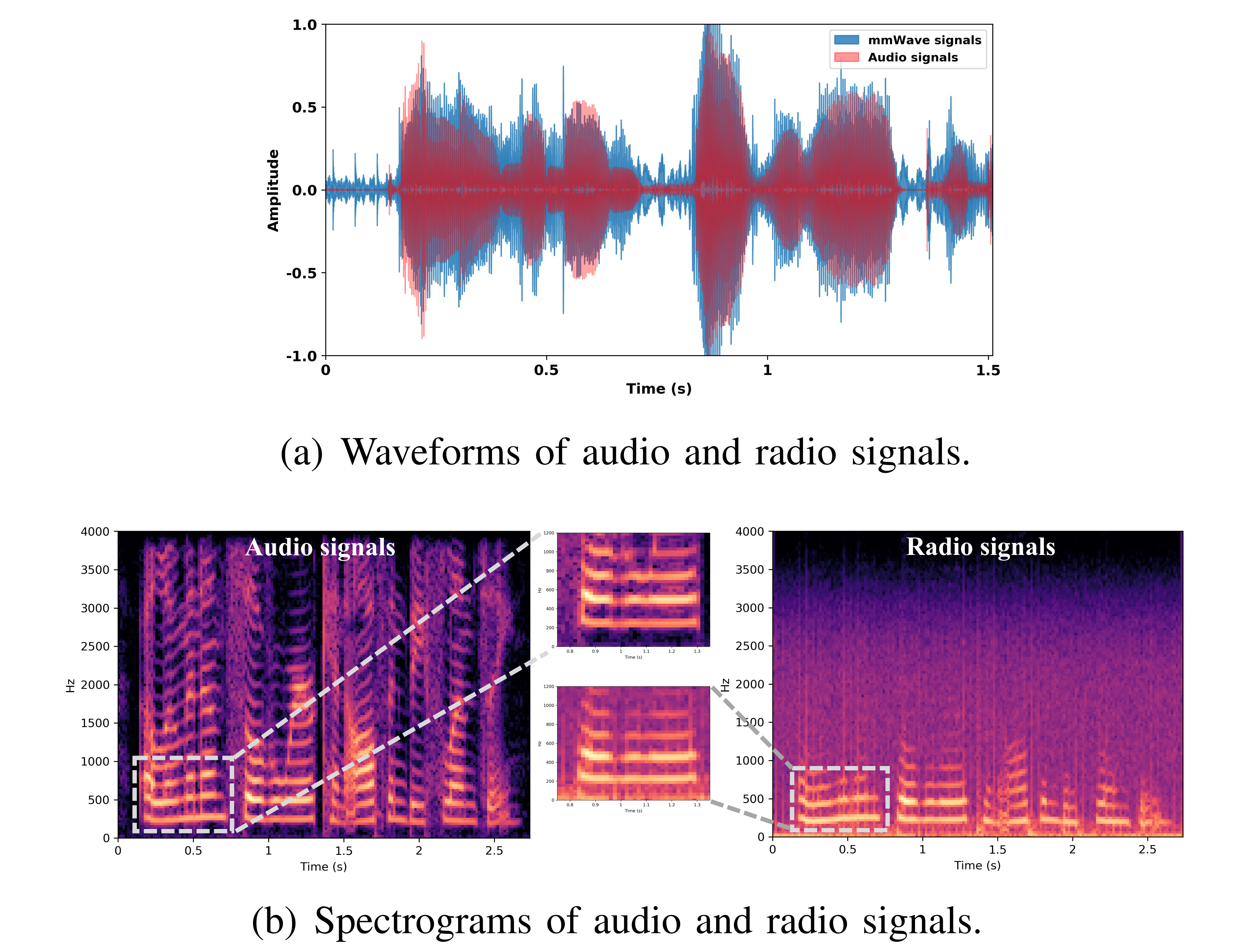
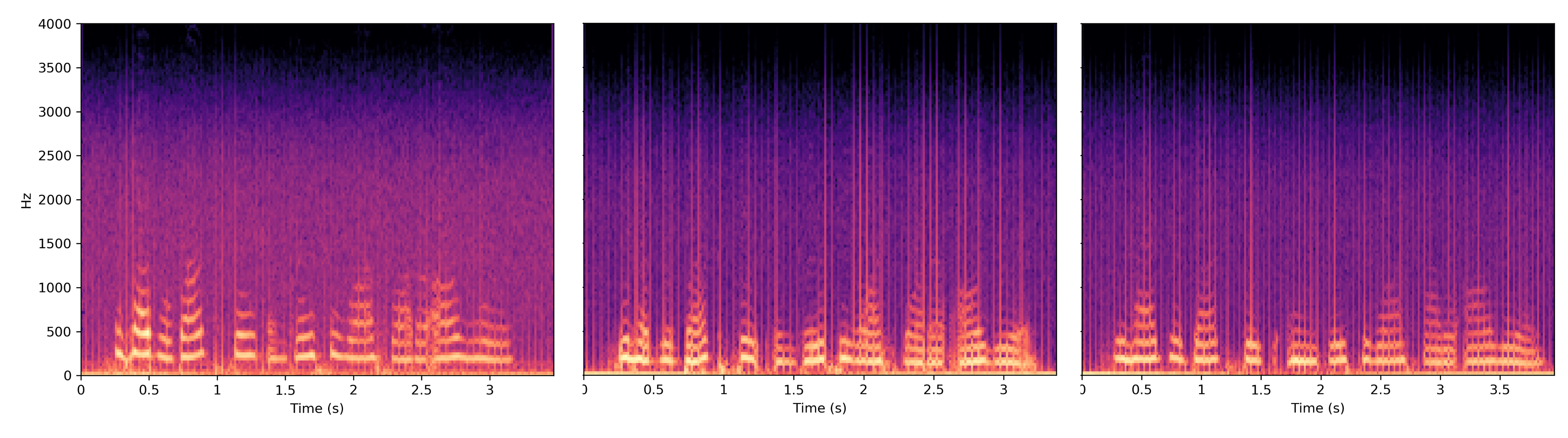
Figure 2 compares an audio waveform and spectrogram with the corresponding radar signal. Their envelopes and lower-frequency structure correlate, while radar measurements lose higher-frequency detail. Figure 3 shows that different voices speaking the same content still produce different timing and spectral patterns.
These examples motivate learning both a cross-modal mapping and speaker-dependent characteristics. Reconstructed high-frequency detail is inferred from learned correlations rather than independently observed in full.
III. System design
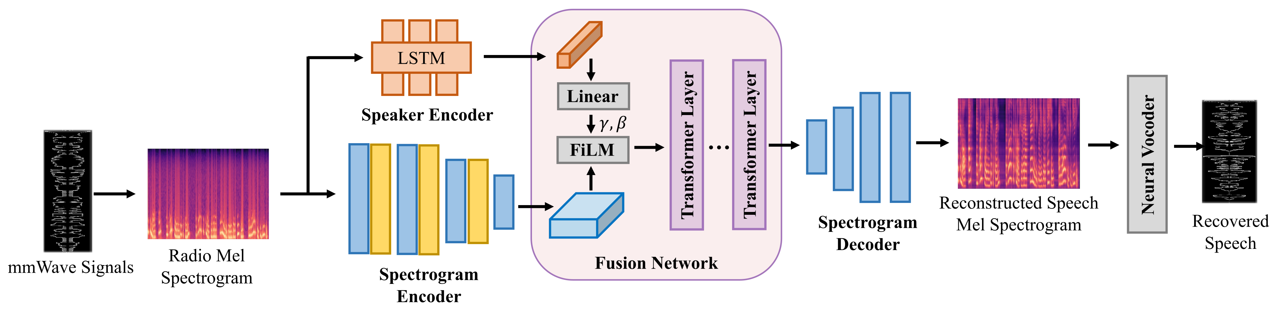
The system separates spectrogram reconstruction from waveform synthesis. Figures 4–7 preserve the complete architecture and conditioning diagrams.
A. System overview
The radio Mel spectrogram enters a speaker encoder and a spectrogram encoder. A fusion network conditions spectrogram features on the speaker embedding and models their global context. A decoder reconstructs a speech Mel spectrogram, and Parallel WaveGAN generates the waveform [32]. No clean target-speaker recording is supplied as a separate conditioning input at inference.
B. Speaker encoder
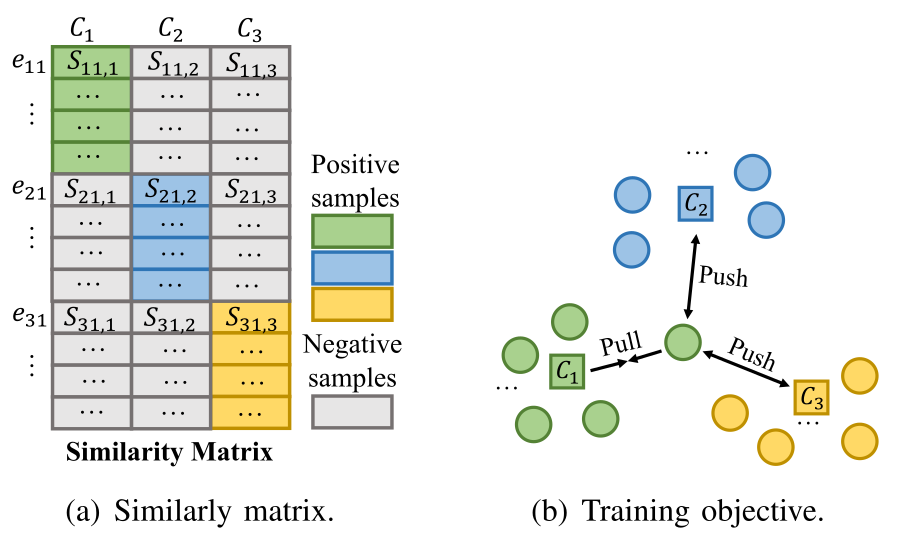
A three-layer LSTM with a projection layer produces normalized speaker embeddings. Training follows generalized end-to-end speaker verification [24]: cosine similarity to each speaker’s embedding centroid is linearly scaled, and the cross-entropy objective in Equation 2 encourages similarity to the correct centroid.
Figure 5 retains the similarity matrix and pull/push illustration. The encoder starts from pretrained speaker-verification weights and is trained on radio signals. During inference, embeddings from fixed-length windows are averaged and normalized, enabling a fixed-dimensional representation of variable-length input.
Equation

C. Spectrogram encoder
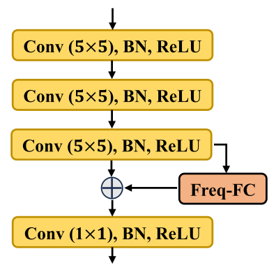
A UNet-style encoder combines convolution with the frequency transformation layer in Figure 6. Local convolution captures nearby time-frequency patterns; a learned fully connected transformation along the frequency axis mixes information from all bands at each time slice. The transformed and local features are concatenated and fused.
This structure provides a learned route for predicting absent high-frequency components from available harmonics. Skip connections retain detail for the paired decoder.
D. Fusion network
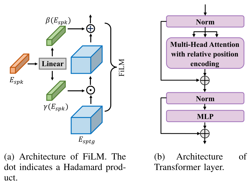
FiLM uses the speaker embedding to generate feature-wise scales and biases for the spectrogram representation [28]. Equation 3 preserves this affine conditioning. The resulting features are divided into patches and processed by Transformer layers.
Relative positional attention, retained in Equation 4, supports varying input lengths [31]. Figure 7 includes both the FiLM and attention-block structures. Conditioning and global context modeling are tested together as the fusion component; their individual effects are not isolated by the reported ablations.
Equations


E. Spectrogram decoder
The decoder reshapes fused patch features and uses PixelShuffle upsampling with encoder skip connections to recover a Mel spectrogram at the input’s time-frequency dimensions. The predicted output is speech-domain spectral information, even though the input comes from radar.
F. Neural vocoder
Parallel WaveGAN synthesizes the waveform from the reconstructed Mel spectrogram instead of reusing contaminated radar phase. Its adversarial training includes a multi-resolution spectral loss. The choice addresses waveform quality; it does not independently verify that inferred speech content is correct.
IV. Implementation
The implementation uses commercial radar hardware, paired speech/radio training data, and pretrained components. The author-accepted manuscript is the source for this edition.
A. Experiment setup
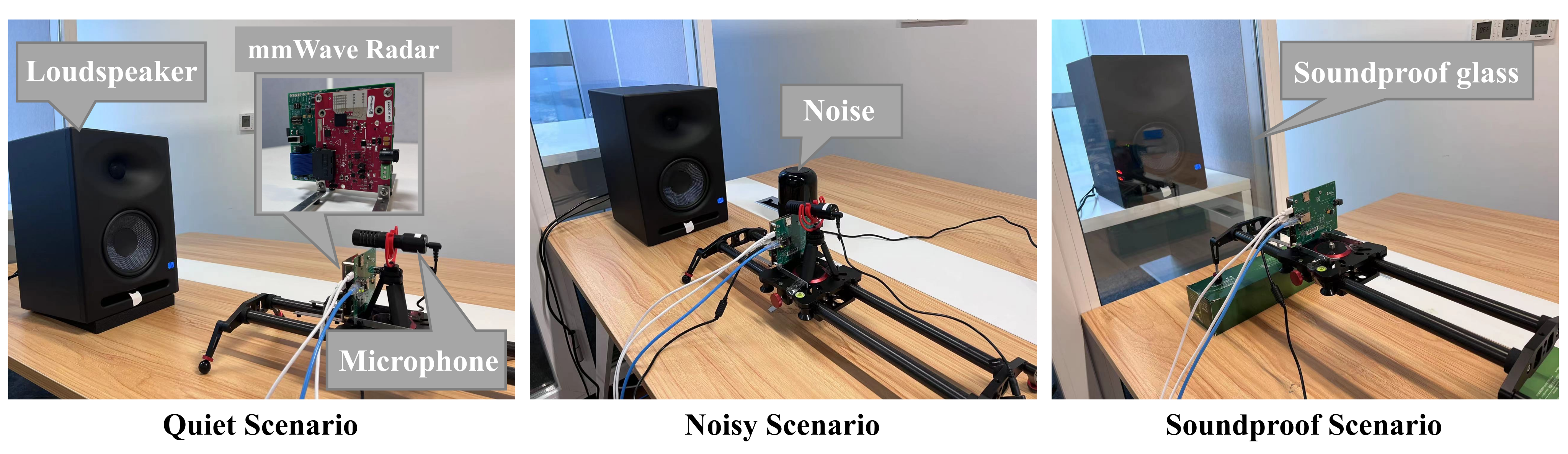
Figure 8 retains the quiet, noisy, and glass-separated collection setups. The main experiments place the stationary loudspeaker and radar 0.5 m apart and play speech at 85 dB SPL. A colocated microphone provides a reference; the noisy condition adds an off-axis noise source.
The radar-derived time series is sampled at 5.1 kHz. Audio and radio recordings are calibrated to a duration mismatch below 10 ms. These controlled acquisition conditions constrain how broadly the reported recovery results can be interpreted.
B. Dataset preparation
TIMIT supplies 6,300 utterances from 630 voices. The seen-speaker split trains on nine utterances per voice and tests on one, yielding 5,670 training and 630 test recordings. The unseen-speaker split trains on all utterances from 567 voices and tests on all utterances from the remaining 63.
The paired radio recordings follow the same splits. Radio signals are resampled and target audio downsampled to 8 kHz, then represented by 80-bin log-Mel features spanning 60–4,000 Hz. Held-out voices test speaker generalization; the split alone does not establish generalization to new languages, spontaneous conversations, or arbitrary sentence content.
C. Network configuration
The speaker embedding has 256 dimensions. The reconstruction network uses three encoder and decoder stages, frequency transformation after each encoder stage, and twelve Transformer layers with eight attention heads. Speaker conditioning supplies scales and biases for 1,024 feature channels.
Radio TransUNet uses AdamW for 130 epochs; the Transformer starts from ImageNet pretraining and the speaker encoder from prior verification training [25]. The vocoder is trained on the corresponding 8 kHz corpus. The implementation references Radio2Speech code. End-to-end latency, memory consumption, and external-pretraining speaker overlap are not separately evaluated here.
V. Evaluation
The evaluation combines objective waveform comparisons, listener ratings, qualitative examples, component ablations, and controlled changes to collection conditions.
A. Evaluation metrics
STOI measures estimated intelligibility and PESQ measures perceptual speech quality; higher is better. LSD measures spectral distance; lower is better. These are waveform-based proxies, not transcription or word-error measurements.
For each speaker split, twenty selected test utterances per method receive naturalness scores from twenty native-speaking listeners through Mechanical Turk. MOS is reported on a five-point scale with 95% confidence intervals. Naturalness ratings should not be read as verified content-recognition accuracy.
B. Baselines
The UNet and conditional-GAN baselines reconstruct a spectrogram and use Griffin–Lim waveform synthesis, following prior radio-speech methods [16] [18]. A constructed TransUNet baseline retains Transformer/UNet reconstruction and Parallel WaveGAN while omitting SPACE’s additional components.
All use the same training and test splits. The comparison covers these implementations, rather than every published eavesdropping system or sensing modality.
C. Overall performance
Separate training and evaluation under the two speaker splits distinguish performance on new utterances from known voices and on entirely held-out voices.
1. Spectrogram examples
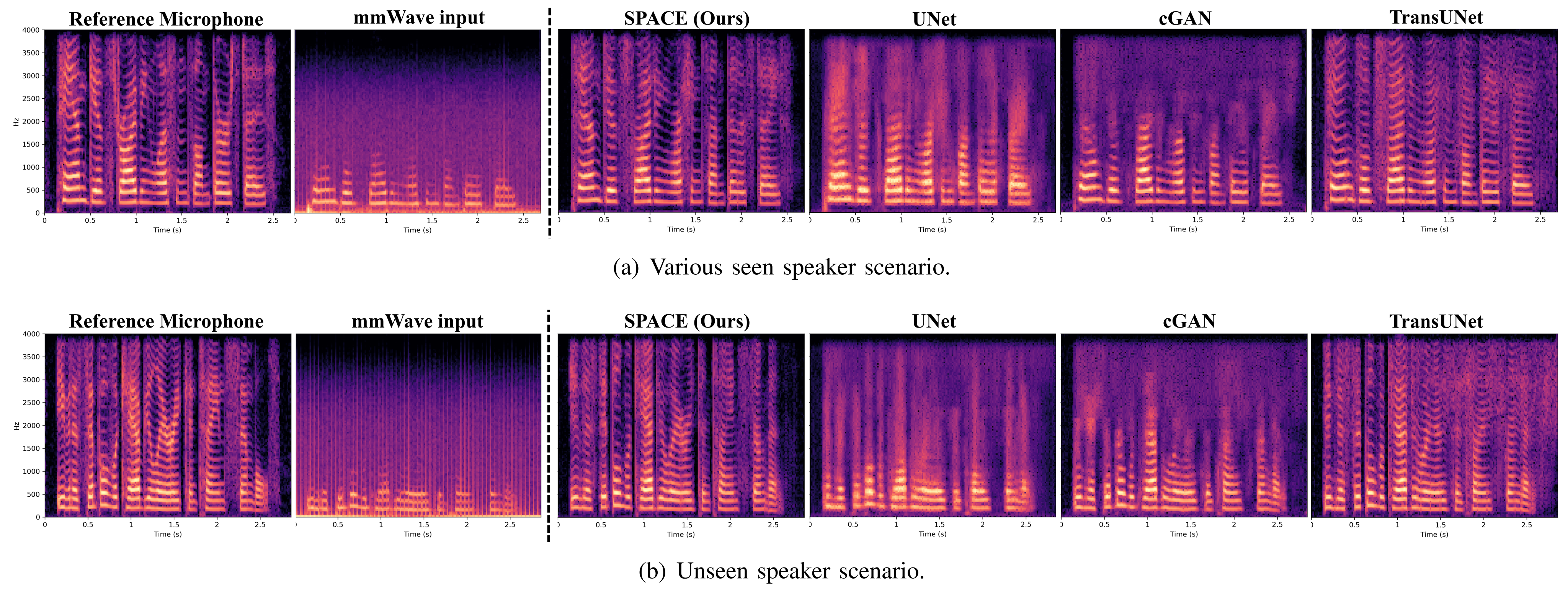
Figure 9 preserves the reference audio, radar input, and four reconstructions for a seen and an unseen voice. SPACE’s illustrated spectrograms retain clearer high-frequency structure. Two selected examples illustrate behavior; they do not establish uniform reconstruction across the test set.
2. Speaker embedding space
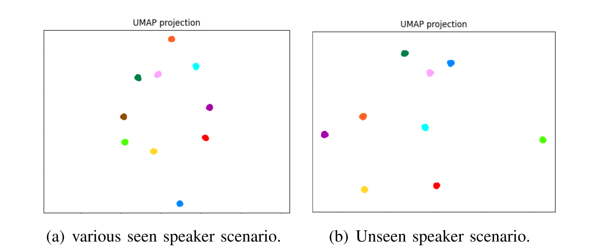
Figure 10 projects speaker embeddings with UMAP, showing separation between the illustrated voices in both splits. This supports the intended representation qualitatively, without providing a separate identification accuracy or proving that the visualization explains the recovery gains.
3. Quantitative evaluation
Table I retains all scores and cross-split differences. SPACE obtains STOI/PESQ/LSD of 0.821/2.129/0.923 for seen voices and 0.814/2.111/0.954 for unseen voices. The corresponding TransUNet values are 0.775/1.959/1.035 and 0.762/1.896/1.072.
SPACE is best on all three metrics in both splits and has smaller STOI and PESQ degradation. The table’s cGAN LSD moves from 1.172 to 1.142, an improvement despite a positive 0.030 in its difference column; therefore the cross-split table should not be read as uniform degradation for every baseline and metric.

4. Listener evaluation
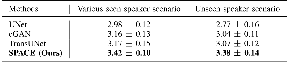
Table II reports SPACE MOS of 3.42 ± 0.10 for seen voices and 3.38 ± 0.14 for unseen voices, compared with TransUNet’s 3.17 ± 0.15 and 3.07 ± 0.12. The result favors SPACE in perceived naturalness for the sampled clips, while the scores remain below the five-point maximum.
D. Complex experimental scenarios
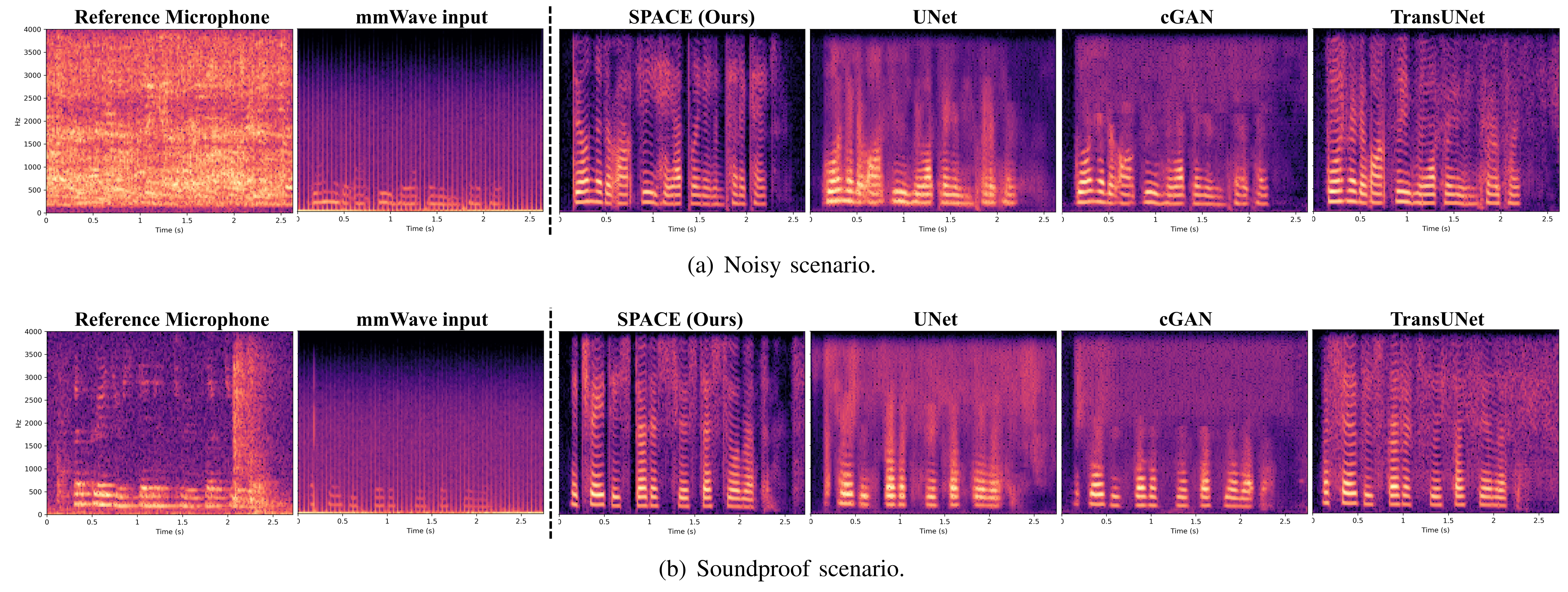
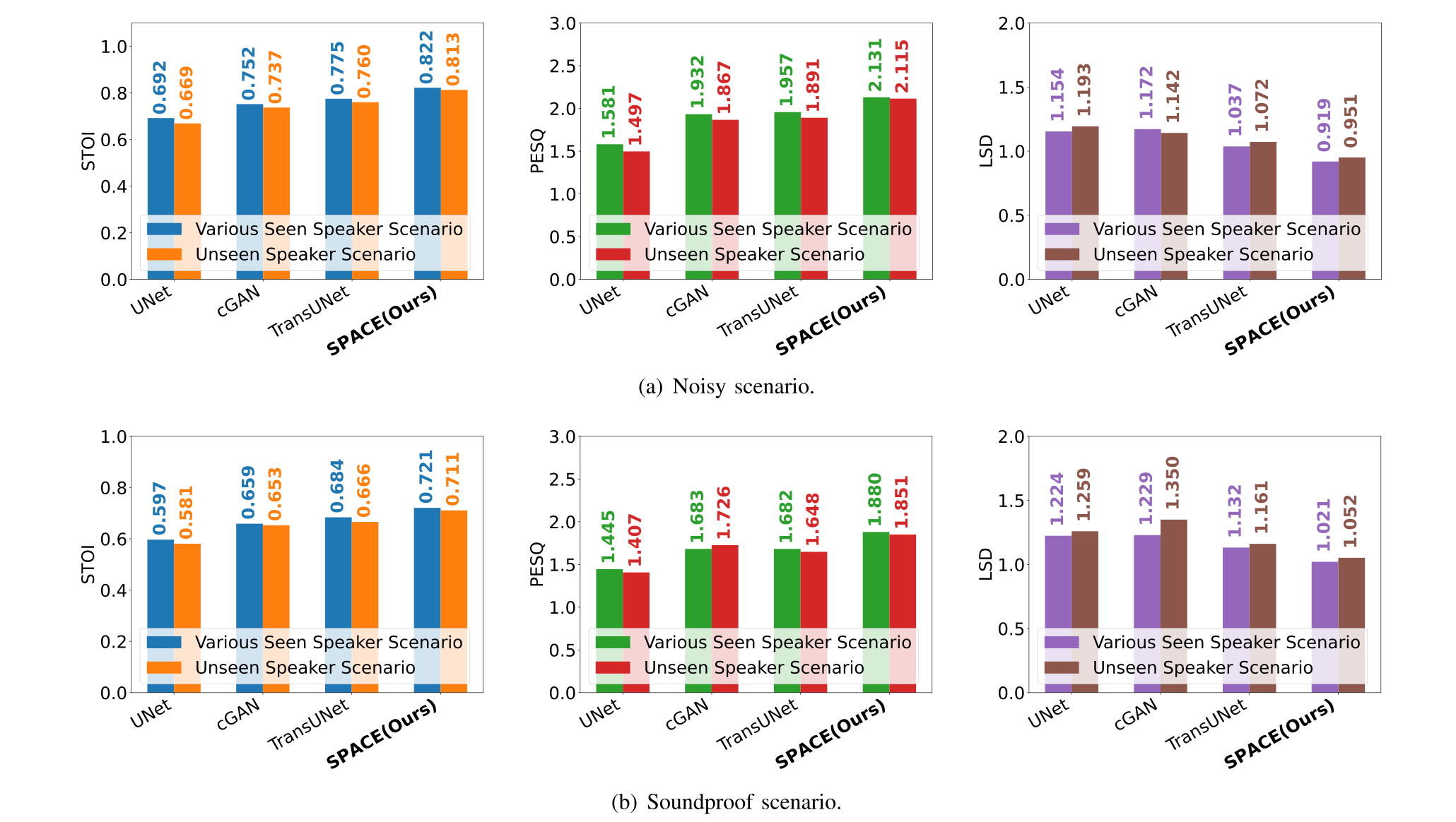
Figures 11–12 retain all spectrogram panels and objective scores for noisy and glass-separated recording. SPACE remains the strongest tested reconstruction method. Noisy-condition scores are close to quiet-condition values, whereas glass separation lowers them: unseen-voice STOI/PESQ/LSD is 0.711/1.851/1.052 through glass, versus 0.813/2.115/0.951 with the added noise.
The discussion’s wording about which condition degrades is inconsistent with the plotted values; these notes follow Figure 12. The experiment demonstrates the tested noise source and barrier, not immunity to all occlusions or environmental interference.
E. Ablation studies
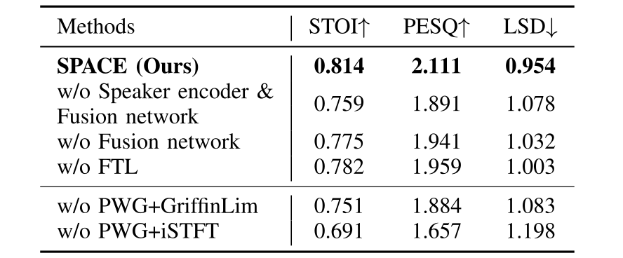
Table III removes components on the unseen-speaker quiet-condition dataset. Without speaker encoding and fusion, STOI falls from 0.814 to 0.759. Replacing fusion with direct concatenation gives 0.775; removing frequency transformation gives 0.782.
Replacing Parallel WaveGAN with Griffin–Lim or inverse STFT gives STOI 0.751 or 0.691, respectively, with corresponding declines in the other metrics. The ablations support the complete design under this protocol, but do not isolate every subcomponent or establish universal superiority of a particular vocoder.
F. Impact of different factors
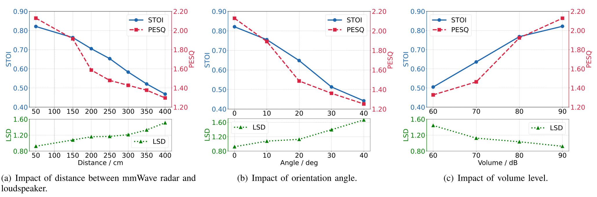
Figure 13 preserves all distance, orientation, and volume curves. These sweeps show that recovery depends strongly on collection geometry and vibration strength. Figures 14–16 retain the loudspeaker, barrier, and room-condition comparisons.
Distance
Performance decreases as separation grows from 0.5 to 4 m. The authors describe relatively intelligible recovery within 2.5 m under the fixed frontal, 85 dB playback setup. This is a conditional result rather than an unrestricted operating range.
Orientation angle
Increasing the angle from frontal alignment to 40° reduces quality. The authors attribute this to reduced visibility of the vibrating membrane and report stronger recovery below 20° under the same short-range, loud-playback conditions.
Volume level
Recovery weakens as playback falls from 90 to 60 dB, with ambient sound around 30 dB. The authors describe comparatively intelligible recovery above 70 dB. Quiet speech and low-vibration sources therefore remain important limits.
Loudspeaker types
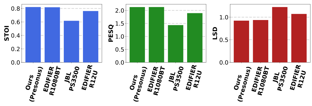
Figure 14 compares four loudspeaker models. Presonus performs best, EDIFIER R1080BT is close, and the other models perform worse. The authors suggest the JBL model’s steel mesh interferes with radio propagation; the experiment does not separately isolate mesh material from other device differences.
Insulation materials
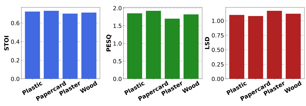
Plastic and paper card allow better recovery than plaster and wood in Figure 15. The authors attribute the difference to attenuation and material structure. Barrier performance is material-dependent, and the provided comparison does not establish general through-wall recovery.
Environmental change
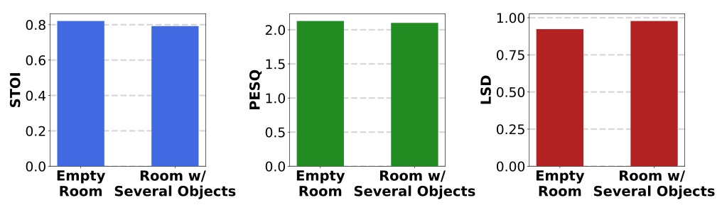
Adding objects to an otherwise empty room slightly worsens the plotted metrics. The authors attribute this to scattering and interference. This two-condition comparison provides limited evidence about environmental variation rather than broad deployment robustness.
A. Acoustic eavesdropping
Prior sensing methods use cameras, light, motion sensors, WiFi, RFID, or millimeter-wave radar. They differ in sensor placement, vibration target, environmental sensitivity, and whether they recover waveforms or recognize words.
SPACE builds on radio-to-speech recovery and adds speaker-conditioned reconstruction. The related-work section explicitly acknowledges earlier unseen-speaker generalization in MilliEar [18], qualifying the broader introduction’s characterization of prior limitations.
B. Speaker adaptation
Feature-based adaptation adds speaker information or normalizes acoustic features; model-based adaptation changes network parameters for the target condition. SPACE primarily uses an embedding from the observed radio signal to condition a shared reconstruction model, transferring the idea of speaker-aware features to cross-modal speech recovery.
VII. Conclusion
The measured gains support speaker conditioning, frequency mixing, and neural waveform synthesis for the tested paired-data task. Remaining gaps include moving and simultaneous speakers, broader environments, direct live-speech recovery, and content-error assessment. Multiple or moving speakers are explicitly left to future work.
Acknowledgments
The work reports support from Hong Kong’s University Grants Committee General Research Fund and Innovation and Technology Commission Fund.