At a glance
Intuition. Suppose a signal has 1,000 transform coefficients but only ten are important. Measuring all 1,000 coordinates can be wasteful. Carefully chosen mixtures of coordinates can retain enough information to reconstruct that sparse signal. The mixtures must distinguish sparse candidates; simply discarding arbitrary coordinates will not do.
Reading the math. In y = Ax, x is the unknown signal, A specifies the measurements, and y contains their observed values. Fewer measurements mean many possible solutions. Minimizing the sum of absolute coefficients, the ℓ1 norm, favors sparse explanations. Recovery depends on the measurement geometry and sparsity; compressible signals generally incur approximation error.
Compressed sensing acquires fewer nonadaptive linear measurements than the ambient signal dimension, then reconstructs by a nonlinear algorithm. The assumption is compressibility in a known orthonormal basis or frame. This paper uses optimal recovery and geometric widths to characterize attainable worst-case error, exhibits random measurement ensembles with the required structure, and proves near-optimal recovery by convex ℓ1 minimization for coefficient classes with 0<p≤1. Its applications are stylized mathematical models, rather than experimental guarantees for arbitrary natural images.
I · Introduction
Transform compression suggests measuring the information a signal retains after compression instead of first acquiring every pixel. The proposed measurements mix many coefficients and are fixed independently of the unknown signal. Sparse structure makes this underdetermined inverse problem recoverable; without a compressibility assumption, fewer linear measurements cannot recover every ambient vector. Nonlinear reconstruction is essential to the proposed acquisition scheme.
I.A · Transform compression background
The coefficient vector belongs to an ℓp ball of radius R in a specified transform. The best N-term approximation retains its largest coefficients, with ℓ2 error bounded by a p-dependent constant times R(N+1)^(1/2−1/p), for 0<p<2. Smaller p imposes stronger compressibility. Bounded-variation images and bump-algebra spectra motivate scale-dependent coefficient bounds; they are particular function classes, not assumptions verified for every measured object.
Equations I.1–I.2




I.B · Optimal recovery and information complexity
An information operator measures n fixed linear functionals; a reconstruction algorithm may be nonlinear. The minimax error takes the worst signal in the specified class and then optimizes jointly over information operators and reconstruction rules. This benchmark distinguishes an existence result for a near-optimal measurement space from an efficient computational procedure using that space.
Equations p.1290–p.1290



I.C · Four surprises and Theorems 1–2
For problem sequences with n tending to infinity and ambient dimension m growing polynomially in n, Theorem 1 gives a compressibility-dependent error scale proportional to R(n/log m)^(1/2−1/p), with constants depending on the growth parameters and p. This matches best-term approximation up to the logarithmic measurement overhead. Theorem 2 bounds the advantage of adaptive linear measurements by a p-dependent constant in this worst-case model. It does not rule out task-specific benefits of adaptivity under other signal classes, noise models, or average-case objectives.
Equations I.3–p.1291




I.D · Geometry and widths
A Gel’fand width asks for a measurement nullspace whose intersection with the signal class has small Euclidean radius. A Kolmogorov width instead measures approximation by a low-dimensional subspace. Theorem 3 connects the former to minimax recovery, exactly in the convex p=1 case and within a p-dependent constant for 0<p<1. Duality and the Kashin–Garnaev–Gluskin result explain the p=1 rate; the paper develops a direct route for the nonconvex coefficient classes.
Equations p.1291–p.1292






I.E · Why existence is insufficient
Classical width arguments establish favorable subspaces without identifying a practical sensing matrix and reconstruction method. The abstract central algorithm finds the center of all admissible signals consistent with the measurements. It is minimax-optimal, but the nonconvex feasible set and unknown class parameters make that description computationally unhelpful. The next results provide concrete matrix conditions and an ℓ1 reconstruction rule.
Equations p.1292–p.1292




I.F · Information and algorithmic results
Conditions CS1–CS3 certify a near-optimal nullspace. Independent uniformly distributed unit-vector columns generate matrices satisfying those conditions with overwhelming probability in the stated asymptotic regime. Measurements combine this matrix with the signal transform. Basis Pursuit minimizes the coefficient ℓ1 norm subject to exact measurement consistency. Theorem 5 combines near-optimal information and near-optimal reconstruction over all 0<p≤1 without requiring the algorithm to know p or R.
Equations p.1292–p.1293





I.G · Potential applications
The introduction forecasts large measurement reductions for modeled spectra, bounded-variation images, and cartoon-like images. These comparisons match a target approximation error to that of a classical sampling scheme, keeping logarithmic factors and class-dependent constants. They are asymptotic acquisition bounds for purpose-designed linear measurements, not claims that arbitrary subsampling or a particular physical scanner automatically achieves the same rates.
I.H · Structure of the argument
The paper separates geometric information bounds, abstract recovery algorithms, tractable Basis Pursuit, function-space extensions, stylized applications, and the random-matrix existence proof. Its concluding comparison with partial Fourier sampling links this width-based approach to contemporary sparse-recovery work.
II · Information
After transferring into coefficient coordinates, the analysis can take the transform to be the identity. The width relative to a matrix is the largest ℓ2 norm of a class member in its nullspace. Minimizing that radius over matrices gives the Gel’fand width. The aim is a nullspace radius within a constant factor of optimal, rather than an invertible map on the entire ambient space.
Equations II.1–p.1293



II.A · Conditions CS1–CS3
For every sufficiently small column subset J, CS1 lower-bounds its minimum singular value; CS2 compares ℓ1 and ℓ2 norms on its column span; CS3 lower-bounds a quotient norm describing representation using complementary columns. The subset threshold is proportional to n/log m, with fixed positive constants independent of the growing dimensions. Theorem 6 asserts that these properties jointly hold for almost all matrices in the specified unit-column ensemble. Merely choosing dimension-dependent tiny constants would not supply the same result.
Equations p.1293–p.1294




II.B · Theorem7: near-optimal CS matrices
The proof orders a nullspace vector by decreasing coefficient size and divides it into its largest entries and tail. Compressibility bounds the tail; CS3 converts its representation cost into an ℓ1 bound on the corresponding measurement vector; CS2 converts that to ℓ2; and CS1 controls the leading coefficients. Combining head and tail gives the desired nullspace-width bound. This is a uniform statement over the specified coefficient class after a matrix satisfies all three conditions.
Equations p.1294–p.1294












III · Algorithms
An information bound alone does not provide an efficient reconstruction. This section first uses abstract feasible-point methods to connect widths with minimax error and prove the introductory theorems. SectionIV then replaces those abstract methods with the tractable convex program.
III.A · Feasible-point methods
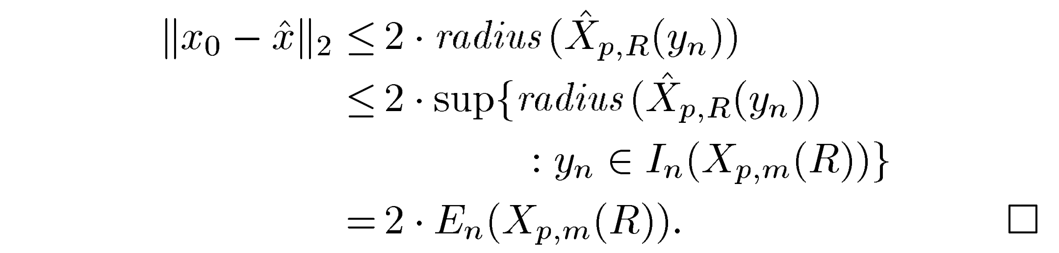
Lemma 3.1 shows that any signal consistent with the measured data and the known class lies within twice the optimal worst-case error when the information operator is optimal. The central algorithm realizes the radius of each measurement fiber; the triangle inequality bounds the distance from another feasible point. The same argument applies with the operator’s own optimal error when its information is only near-optimal. Minimizing the coefficient ℓp norm avoids knowing R, but remains nonconvex when p<1.
Equations p.1294–p.1295









III.B · Proof of Theorem3
For 0<p<1, the p-triangle inequality controls the quasi-norm of a scaled difference of two signals from the same measurement fiber. That difference lies in the nullspace, so the Gel’fand radius bounds it. Comparing the fiber radius with the nullspace radius gives the stated p-dependent bracketing. This is the mechanism extending the convex optimal-recovery relation to the nonconvex ℓp balls.
Equations p.1295–p.1295








III.C · Proof of Theorem1
For p<1, entropy-number lower bounds and Carl’s comparison inequality give one side of the minimax rate. The random-matrix construction and the CS-width theorem give the matching upper order; feasible-point recovery transfers it into an algorithmic error bound. Constants and the polynomial dimension-growth regime remain part of this asymptotic comparison.
Equations p.1296–p.1296





III.D · Proof of Theorem2
Run an adaptive linear-measurement strategy on the zero signal. All class members in the resulting nullspace produce the same observations along that branch. Their remaining uncertainty lower-bounds the strategy’s minimax error by a Gel’fand width. Comparing with the nonadaptive width bound limits the advantage of adaptivity in this symmetric worst-case setting.
Equation p.1296

IV · Basis Pursuit
The previous least-ℓp method depends on p and becomes a nonconvex optimization for p<1. Basis Pursuit removes both difficulties by using the same ℓ1 objective across all the compressible classes studied here.
IV.A · The case p=1
Split each real coefficient into positive and negative parts to write ℓ1 minimization as a linear program. For p=1, the feasible-point argument immediately makes this procedure near-optimal with near-optimal information. The source’s relative-error illustration additionally needs a relation between the signal norm and its ℓ1 bound: an absolute bound in terms of R does not alone establish a relative error bound for arbitrarily small signals.
Equations p.1296–p.1296






IV.B · Relation between ℓ1 and ℓ0 minimization
Theorem 8 proves that a sufficiently sparse exact solution is the unique minimizer of both the counting objective and the ℓ1 program when CS1–CS3 hold. Lemma 4.1 bounds how much ℓ1 mass any nullspace vector can concentrate on a small set. If that fraction is below one half on the true support, every nonzero feasible perturbation increases the objective. This nullspace property, rather than sparsity alone, explains exact recovery.
Equations p.1297–p.1297











IV.C · Theorem9: near-optimality for 0<p<1
Lemma 4.2 proves an ℓ1 stability estimate when the coefficient tail outside a chosen support is small and nullspace concentration there is below one half. The proof uses optimality of the ℓ1 solution and separates support and complement. Theorem 9 combines that stability estimate with compressibility and the CS-width bound, yielding an ℓ2 approximation rate for nonsparse but compressible vectors. This coefficient-tail stability argument should be distinguished from a complete general theorem for arbitrary measurement noise.
Equations p.1297–p.1298
















V · Immediate extensions
The proof uses structural properties of the transform and coefficient tails that extend beyond a finite orthonormal basis. The two following extensions identify which ingredients must be preserved.
V.A · Tight frames
Parseval tight frames preserve the norm and reconstruction identities required by the width and Basis Pursuit arguments. The paper therefore extends the scheme to redundant coefficient systems such as curvelets. A referee’s observation also permits general frames with constants depending on their frame bounds; redundancy does not remove the need to account for those bounds.
Equations p.1298–p.1298


V.B · Weak ℓp balls
A weak-ℓp constraint bounds the decreasing rearrangement of coefficient magnitudes rather than their full ℓp sum. It supplies the same type of best-term tail estimate needed in the proofs, so the recovery arguments extend to these classes. The weak quantity is a quasi-norm in the relevant range, and the constants and admissible p range remain part of the estimates.
Equations p.1298–V.1


VI · Stylized applications
Each example first proves coefficient compressibility for a specified function class and then balances coarse direct samples against compressed fine-scale measurements. The conclusions compare acquisition complexity at matched approximation error. They are mathematical constructions, not reported sensor trials.
VI.A · Bump algebra
For modeled spectra, smooth-wavelet coefficients decay across scales in ℓ1. Coarse scaling coefficients are measured directly; finer detail coefficients are acquired through a CS matrix and reconstructed by Basis Pursuit. Balancing their errors gives roughly a cube-root reduction in the sample count relative to the classical scheme, up to logarithmic factors. The sensing kernels are linear combinations of wavelets, rather than simply a small subset of point samples.
Equations p.1299–VI.1







VI.B · Bounded-variation images
The two-dimensional Haar construction uses bounded variation and a bounded signal amplitude to control coefficients. Again a coarse direct component is combined with compressed detail measurements. The resulting error matches the classical sampling order with roughly a square-root number of measurements, retaining the logarithmic factors shown in the source. The image-class assumptions and the chosen multiscale measurement operator are essential.
Equations p.1299–p.1300







VI.C · Piecewise C² images with C² edges
The cartoon model consists of bounded smooth regions separated by controlled smooth curves. Curvelet tight frames provide weak-ℓ(2/3) coefficient control. Combining that redundancy-aware representation with the weak-space extension leads to roughly a fourth-root sample count at comparable error, with logarithmic factors. It is a specialized regularity model and does not assert the same rate for arbitrary textured imagery.
Equations p.1300–p.1300









VII · Nearly all matrices are CS matrices
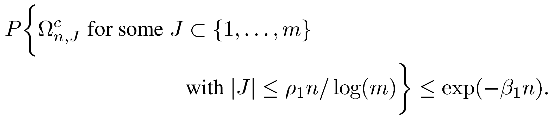
Theorem 10 restates the existence result for columns sampled independently and uniformly from the unit sphere, with polynomially growing ambient dimension. The proof separately makes CS1, CS2, and CS3 likely and intersects their events. Failure probabilities decay exponentially for suitable fixed constants and sufficiently large dimensions. This is a probability statement over the prescribed matrix ensemble, not a certificate for every realized matrix.
Equations p.1301–p.1301


VII.A · Controlling the minimum eigenvalue
Lemmas7.1–7.3 combine a fixed-subset random-matrix singular-value bound with a counting and union-bound argument over all small subsets. Restricting subset size to order n/log m keeps the combinatorial cost below the exponential probability bound. The resulting simultaneous lower singular-value control supplies CS1.
Equations p.1301–p.1301








VII.B · Spherical sections
The almost-spherical-section phenomenon compares ℓ1 and ℓ2 norms on random low-dimensional spans. Lemma 7.5 gives a fixed-subset estimate with explicit parameter constraints; Lemma 7.3 upgrades it to every admissible column subset. Lemma 7.4 therefore supplies CS2. Concentration and counting must be balanced; a typical individual span alone would not prove the uniform condition.
Equations VII.1–p.1302







VII.C · Quotient norms and duality
The quotient ℓ1 minimization problem has a dual feasible region defined by correlations with complementary columns. Lemma 7.6 constructs vectors close to scaled sign patterns while controlling those correlations. Pairing such a vector with the target gives a lower bound on the primal representation cost, hence CS3. The individual embedding estimate is upgraded to a uniform one using a bound on the number of realizable sign patterns.
Equations p.1302–p.1303

















VII.D · Individual sign-pattern embedding
The remaining proof constructs a nearby dual-feasible vector and controls its trajectory. The algorithmic construction, its pathwise bounds, and the large-deviation calculation are separate steps; all three are needed for the uniform quotient-norm argument.
VII.D.1 · An embedding algorithm
Begin from an approximate sign-pattern vector. At each stage identify columns with excessive correlation and project out their span. Thresholds approach the dual feasibility boundary, and the procedure terminates after at most n stages. Termination certifies feasibility; the separate probability analysis is needed to show that the cumulative displacement remains small.
Equations p.1303–p.1303





VII.D.2 · Analysis framework
The proof tracks the norms of successive corrections and the number of remaining high-correlation indices. Geometric bounds on these quantities imply a bound on total displacement. A sequence of good trajectory events is arranged so that controlling their conditional failure probabilities yields the individual embedding result.
Equations p.1303–p.1303








VII.D.3 · Large deviations
Minimum-eigenvalue control ensures that the required projections remain well conditioned. The analysis reduces trajectory failures to Gaussian tail counts and truncated-square sums. Lemma 7.8 bounds these events exponentially; the chosen thresholds and constants leave a positive exponent. Some supporting distributional arguments are imported from the companion paper, as the source explicitly notes.
Equations p.1303–p.1304



















VIII · Conclusion
The completed scheme joins compressibility, a suitable sensing matrix, and convex reconstruction. The practical promise is reduced acquisition at an error rate close to the optimal-recovery benchmark. Its theorem statements retain their signal-class, matrix, exact-data, and asymptotic assumptions.
VIII.A · Summary
The measurement operator composes the CS matrix with a known coefficient transform; reconstruction minimizes the transformed ℓ1 norm under measurement constraints. The paper derives approximation bounds and motivates imaging and spectroscopy applications. Its broad concluding mention of small measurement errors goes beyond the main exact-consistency statements developed here; those results should not be read as an unrestricted noise-robustness theorem.
Equation p.1304

VIII.B · Alternative formulation
Theorem 11 shows that CS1–CS3 are sufficient rather than uniquely necessary. A small nullspace-concentration bound on thin coordinate sets and a favorable ℓ1-ball width suffice for the same recovery argument. This formulation separates the geometric properties actually used from one particular probabilistic construction.
Equations VIII.1–p.1305



VIII.C · Partial Fourier ensembles
The discussion connects the framework with Candès–Romberg–Tao exact sparse Fourier recovery and Gilbert and collaborators’ near-best Fourier approximation work. It distinguishes uniform and nonuniform row-sampling distributions and the different concentration and width properties obtained from them. These links motivate structured sensing operators, rather than making every partial Fourier matrix satisfy the same guarantee. [13, 12]
Note added in proof
The historical note points to emerging numerical and sensor studies and related data-stream ideas. It records the state of the surrounding work at publication. Those announcements are not additional experiments conducted or quantified in this article.
Acknowledgment
Donoho credits conversations with Emmanuel Candès about undersampled imaging and partial Fourier results, and with Anna Gilbert about nonadaptive Fourier approximation and data streams. These acknowledgments distinguish the present width-based development from related contemporary contributions.