This edition follows the September 2004 arXiv v1 manuscript, including its proofs and appendix. The DOI identifies the later February 2006 journal publication; version-specific wording and formulas here follow the reviewed manuscript. Author affiliations are Caltech and UCLA. The source’s acknowledgments credit supporting institutions and earlier discussions; they are not experimental results.
At a glance
Intuition. A Fourier coefficient describes one frequency component of a signal. This paper asks whether observing a randomly selected subset of those components can still identify the original signal. Sparsity supplies the missing information: the decoder searches among signals with very few nonzero entries rather than among all possible signals.
Reading the math. N is the full signal length, T is its nonzero support, and Ω is the set of measured frequencies. The recovery program matches the observed frequencies while minimizing the sum of absolute signal values. Think of the measurements as clues that must uniquely distinguish the sparse answer. The stated guarantee is probabilistic and noiseless; image extensions instead exploit sparse changes between pixels.
For a fixed sparse signal, randomly sampled Fourier coefficients can determine its exact ℓ1 reconstruction with high probability once the expected measurement count is sufficiently large relative to support size and log signal length. The proof constructs a dual trigonometric polynomial and controls random-matrix moments. Sparse differences motivate total-variation extensions and phantom-image demonstrations. Exact noiseless recovery, random sampling, and fixed-signal probability are central assumptions; “robust” in the title does not mean that this manuscript proves a complete arbitrary-noise recovery theorem.
Equations
1 Introduction
Incomplete Fourier data leave an underdetermined inverse problem. Sparsity supplies additional structure, while convex minimization chooses a low-complexity feasible signal without knowing its support in advance. The paper separates information-theoretic uniqueness, computational recovery, and probabilistic sampling guarantees.
Equation
1.1 A puzzling numerical experiment
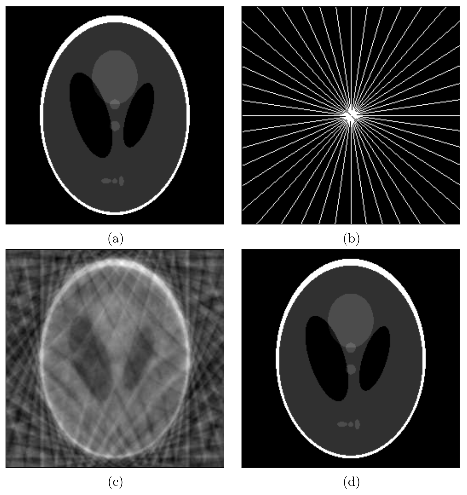
A 512×512 phantom is sampled along 22 approximately radial Fourier lines. Setting unseen Fourier values to zero produces strong artifacts; minimizing discrete isotropic total variation recovers the displayed piecewise-constant phantom exactly in the reported numerical experiment. Figure 1 retains the original, sampling mask, minimum-energy reconstruction, and TV reconstruction. Radial sampling in this illustration is different from the independent Bernoulli Fourier sampling of the main theorem, and a successful synthetic phantom is not a general medical-imaging validation.
Figure 1: Example of a simple recovery problem. (a) The Logan-Shepp
phantom test image. (b) Sampling ’domain’ in the frequency plane;
Fourier coefficients are sampled along 22 approximately radial
lines. (c) Minimum energy reconstruction obtained by setting
unobserved Fourier coefficients to zero. (d) Reconstruction
obtained by minimizing the total-variation, as in (1.1).
The reconstruction is an exact replica of the image in (a).Equations 1.1
(1.1)
1.2 Main Results
For prime signal length, Theorem 1.1 gives uniqueness among sufficiently sparse signals from an arbitrary frequency subset, with a sharp support-count obstruction beyond that threshold. It relies on injectivity of square Fourier minors and does not itself give an efficient reconstruction algorithm. The ℓ0 search is combinatorial; the proposed ℓ1 program is convex. Theorem 1.3 instead fixes a signal and draws each frequency independently with probability τ: support size is at most α(M)τN/logN, and recovery succeeds with probability 1−O(N^−M). This is not an assertion that one draw simultaneously recovers every signal of that sparsity. The proof’s explicit constants are conservative and carry the sampling-parameter conditions shown later.
Equations 1.2
(1.2)
Theorem 1.1
Suppose that the signal length is a prime integer. Let be
a subset of , and let be a vector supported
on such that
Equation 1.3
(1.3)
Then can be reconstructed uniquely from and . Conversely, if is not the set of all
frequencies, then there exist distinct vectors such that
and such that
.
Lemma 1.2
([18], Corollary 1.4)
Let be a prime integer and be subsets of
. Put (resp. ) to be the
space of signals that are zero outside of
(resp. ). The restricted Fourier transform is defined
as
Equation
If , then is a
bijection; as a consequence, we thus see that is injective for and surjective for
.
Clearly, the same claims hold if the
Fourier transform is replaced by the inverse Fourier
transform .
Equations 1.4–1.8
(1.4)
(1.5)
(1.6)
(1.7)
(1.8)
Theorem 1.3
Let be a discrete signal and be the random set
defined in (1.7). For a given accuracy parameter ,
if is supported on and
Equation 1.9
(1.9)
then with probability at least , the minimizer to the problem
(1.5) is unique and is equal to .
1.3 For Almost Every Ω
Two counterexamples explain why the sampling assumptions matter. A Dirac comb can have all its informative Fourier coefficients omitted, making recovery impossible even before choosing an algorithm. A carefully placed box signal and a Fourier-invisible perturbation can also defeat ℓ1 minimization. Such structured bad subsets do not contradict a high-probability result over random subsets. Sparsity alone does not make every undersampled Fourier system recoverable.
1.4 Extensions
A piecewise-constant signal has sparse first differences, so recovery can be expressed by total-variation minimization, with its mean fixed separately. Higher-dimensional sparse recovery uses the same strategy; detailed proofs of some extensions are omitted in the source. The printed one-dimensional conversion contains a multiplier inconsistency: after deriving δ̂=(1−e^−iω)ĝ, it defines υ as the reciprocal but writes υf̂ in the equivalent constraint. The original formulas remain unchanged; a direct implementation should use the multiplier implied by the displayed difference identity.
Equations 1.10
(1.10)
Corollary 1.4
Put . Under the assumptions of
Theorem 1.3, the minimizer to the problem (1.10)
is unique and is equal with probability at least
—provided, of course, that be adjusted so that
.
Theorem 1.5
Put . We let be a
discrete signal and be the random set defined as in
(1.7). Assume that for a given accuracy parameter ,
is supported on obeying (1.9). Then with
probability at least , the minimizer to the problem
(1.5) is unique and is equal to .
1.5 Relationship to Uncertainty Principles
A sufficient nullspace condition says that no nonzero Fourier-invisible perturbation can place half its ℓ1 mass on the signal support. The triangle inequality then makes every feasible perturbation increase the objective. Classical deterministic uncertainty bounds imply only much more restrictive support sizes in the regime of interest. The paper therefore pursues dual certificates and random sampling rather than relying only on that deterministic estimate.
Equations
1.6 Robust Uncertainty Principles
The proposed robust uncertainty principle concerns typical support pairs, contrasting them with special extremal configurations such as combs. Its stronger scale is probabilistic, with a failure level controlled by the chosen accuracy parameter. The source sketches this broader interpretation rather than developing all its consequences; its title should not be read as a uniform bound for every support pair or a theorem about measurement-noise robustness.
Equations 1.11–1.12
(1.11)
(1.12)
1.7 Connections with existing work
The work builds on Basis Pursuit and sparse dictionary-representation results, but recovers an incompletely observed signal rather than merely choosing a sparse expansion of a fully known vector. Random-matrix estimates permit substantially different sampling regimes. Connections to spectral estimation and sublinear Fourier approximation are discussed with care: here the frequency observations are externally specified, and producing a complete length-N reconstruction itself precludes a sublinear output algorithm. [3, 7]
Equation 1.13
(1.13)
2 Strategy
The recovery proof needs both injectivity on the true support and a dual polynomial with the correct signs on that support and magnitude strictly below one elsewhere. These conditions make the feasible optimum unique. The remaining argument shows they hold with high probability for the proposed random-frequency model.
2.1 Duality
For a real signal the program can be written using nonnegative positive and negative parts; its dual motivates the certificate. Lemma 2.1 states the corresponding complex-valued result. A certificate supported in the observed Fourier set, together with injectivity on the signal support, proves uniqueness by an ℓ1 inequality and Parseval orthogonality. The proof checks the equality case: a competing optimum must vanish off the support and then injectivity forces it to coincide with the signal. The original statement is retained with its exact assumptions.
Equations 2.1–2.7
(2.1)
(2.2)
(2.3)
(2.4)
(2.5)
(2.6)
(2.7)
Lemma 2.1
Let . For a vector , define the
’sign’ vector by when and otherwise. Suppose there exists a
vector whose Fourier transform is supported in
such that
Equation
and
Equation
•
Then if is injective, the
minimizer to the problem (1.5) is unique
and is equal to .
•
Conversely, if is the unique minimizer of , then
there exists a vector with the above properties.
Equations
2.2 Architecture of the Argument
Fix the signal and its support T. Concentration first controls the random sample count. An off-diagonal operatorH removes the deterministic diagonal of the restricted Fourier Gram matrix. Inverting its support restriction yields the polynomial in Eq 2.11, which automatically has the required Fourier support and interpolates the signal signs. The two remaining tasks are bounding that inverse and controlling the polynomial outside T. Degree-of-freedom intuition alone does not establish the strict off-support inequality.
Equations 2.8–2.11
(2.8)
(2.9)
(2.10)
(2.11)
3 Construction of the Dual Polynomial
The construction uses high moments of a random matrix to obtain invertibility and high moments of a truncated Neumann series to control the off-support certificate. The source keeps the numerical constants explicit, sacrificing sharpness for a quantitative failure bound.
3.1 Invertibility
A direct Frobenius-norm estimate only handles very small supports. Raising the self-adjoint matrix to a high power exposes cancellations from random frequency selection. Theorem 3.1 bounds the expected trace of an even power; Markov’s inequality then controls the operator norm and hence invertibility of the restricted Gram matrix. Theorem 3.3 supplies a technical estimate for τ≤0.44 and moment order at least4, and Corollary 3.4 converts it to a polynomially small failure probability. Printed inequalities and parameter restrictions are retained rather than simplified into a universal constant.
Equation
Theorem 3.1
Put for short, where is the operator defined by
(2.10). Set and let
Equation
Then
Equation 3.1
(3.1)
Equations 3.2–3.3
(3.2)
(3.3)
Corollary 3.2
Suppose . Then for any
, we have
Equation
Equations 3.4–3.5
(3.4)
(3.5)
Theorem 3.3
Assume that , say, and suppose that obeys
(3.5). Then (3.3) holds for any , and
therefore
Equation 3.6
(3.6)
Equations
Corollary 3.4
Take . We see from the Neumann series that the
operator is invertible
with probability at least since is the identity on vectors supported on .
3.2 Magnitude of the polynomial on the complement of T
A finite geometric-series identity separates the inverse into a truncated Neumann sum and a small remainder. An operator-norm or high-power bound controls the remainder; a dimension-dependent conversion then bounds its infinity norm. This reduction leaves the truncated series as the principal obstacle. The displayed Frobenius-norm assumptions are part of the source’s chosen sufficient events, not a free consequence of matrix invertibility alone.
Equations 3.7–3.8
(3.7)
(3.8)
3.3 Estimating the truncated Neumann series
The off-support polynomial splits into a main truncated term P0 and a remainder P1. Lemma 3.5 bounds moments of individual series terms using the same combinatorial machinery as the matrix moment theorem. Lemma 3.6 groups term orders and applies probability bounds so that the main contribution stays below 0.91; Lemma 3.7 controls the remainder by 0.09 under its additional parameter condition. Their combination gives strict certificate control with high probability. The numerical split is one proof choice, not an empirical phase transition.
Equations
Lemma 3.5
Set . Then obeys the same estimate as
that in Theorem 3.1 (up to a multiplicative factor
), namely,
Fix . Suppose that obeys (3.5) and let
be the set where
with as in (2.9). For each , there is a set with the property
Equation
and
Equation
As a consequence,
Equation
and similarly for .
Equations 3.11–3.12
(3.11)
(3.12)
Lemma 3.7
Fix . Suppose that the pair obeys . Then
Equation
on the event , for
some obeying .
Equation
3.4 Proof of Theorem 1.3
The proof chooses a moment order proportional to(M+1)logN and a numerical parameter 0.42, combines invertibility and certificate events, and derives a conservative support constant of order 1/[29.6(M+1)]. Intermediate failure estimates include logarithmic factors, and several printed narrative sentences write a small failure probability where the surrounding argument requires a large success probability. The reading claim is the stated high-probability recovery theorem with its full assumptions, not those isolated wording slips.
Equations 3.13
(3.13)
4 Moments of Random Matrices
The technical core expands expected traces by grouping repeated sampled frequencies. Dependence caused by repeated indices prevents treating every factor as independent. Set partitions, inclusion–exclusion, Stirling numbers, and convex bounds organize the surviving terms.
4.1 A First Formula for the Expected Value of the Trace of ( H 0 ) 2 n
Expand the trace into closed index walks and products of Fourier coefficients. A partition records which frequency indices coincide. Bernoulli sampling contributes a power ofτ equal to the number of distinct frequency classes. Keeping that collision pattern is essential: multiplying independent expectations for every occurrence would give the wrong moment. The two-index example illustrates why sums with distinctness exclusions are awkward.
Equations 4.1–4.2
(4.1)
(4.2)
4.2 Inclusion-Exclusion formulae
Lemma 4.1 rewrites sums over exactly specified frequency-collision patterns as signed sums over coarser equality constraints. Its factorial coefficients account for ways classes can merge. The inductive proof adds the final index either as a singleton or into an existing class, weighting repeated descriptions correctly. Removing inequality exclusions lets the Fourier sums factor and subsequently vanish unless linear constraints on signal indices hold.
Lemma 4.1 (Inclusion-Exclusion principle for equivalence classes)
Let and be non-empty finite sets. For any equivalence class
on , we have
Equation 4.3
(4.3)
Equations 4.4–4.5
(4.4)
(4.5)
4.3 Stirling Numbers
Stirling numbers count partitions with a specified number of classes. Their recurrence leads to a generating identity for the auxiliary functionsFn(τ), valid in the statedτ<1/2 range. Lemma 4.3 bounds the alternating series using the location of its largest term. These functions retain the repeated-frequency contribution after inclusion–exclusion; treating them as independent entries of a generic random matrix would miss the Fourier structure.
Equations 4.6
(4.6)
Lemma 4.2
For any and , we have the identity
Equation 4.7
(4.7)
Note that the condition ensures that the right-hand side is convergent.
Equations 4.8
(4.8)
Lemma 4.3
Let and . If , then we have .
If instead , then
Equation
Equation
4.4 A Second Formula for the Expected Value of the Trace of H 0 2 n
The weighted partition identity factors each contribution into one auxiliary function per class. Summing frequencies then enforces a linear constraint for each class: a Fourier sum is eitherN or zero. Singleton classes contribute nothing because adjacent signal indices are required to differ. Lemma 4.5 is the resulting exact combinatorial trace formula and serves as the basis of the later estimates.
Equation
Lemma 4.4
Equation 4.9
(4.9)
Equations 4.10
(4.10)
Lemma 4.5
For every equivalence class , let
. Then
Equation 4.11
(4.11)
4.5 A First Bound on E [ Tr ( H 0 2 n ) ]
The proof bounds how many signal-index tuples satisfy the partition constraints and counts partitions without singleton classes. Lemma 4.6 supplies a factorial-type upper bound involving the golden ratio. The manuscript’s printed recurrence Eq 4.12 omits the factork multiplyingP(n−1,k) for partitions into k nonsingleton blocks; for example P(5,2)=10 while the printed right side gives7. The original equation is preserved, and the prose should be read as the intended counting strategy rather than a line-by-line verification of that printed recurrence.
Equations 4.12–4.13
(4.12)
(4.13)
Lemma 4.6
The numbers obey
Equation 4.14
(4.14)
Equation
4.6 Convex analysis
A convex function attains the displayed simplex maximum at a vertex; the log-convex version bounds products. Applying that principle to the class-size factors reduces their worst configuration to extreme class sizes. A further discrete-convexity argument reduces the remaining partition-count sum to its endpoint terms. The source leaves one elementary inequality verification to the reader; the original formulas preserve its exact parameter and index conventions.
Lemma 4.7
Let be a convex function on , say.
Consider the problem
Equation 4.15
(4.15)
Then the maximum value is obtained by allocating one to
1 and all the others to 0, i.e. .
Equations
Corollary 4.8
Suppose that is a convex function on
, say, and consider
Equation 4.16
(4.16)
Then the maximum value is obtained by allocating one to
1 and all the others to 0, i.e. .
Equations 4.17–4.20
(4.17)
(4.18)
(4.19)
(4.20)
Lemma 4.9
For each , obeys
Equation
Equations
4.7 Proof of Theorem 3.1
The endpoint estimates yield the two termsan andbn in Theorem 3.1. Combining them with the partition count completes the stated moment bound. This closes the random-matrix component used earlier for invertibility and certificate construction, subject to the source’s printed technical formulas and the qualifications noted alongside them.
Equations
5 Numerical Experiments
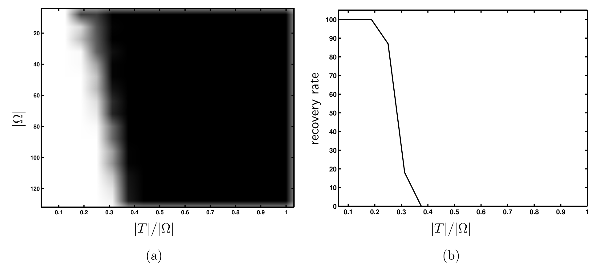
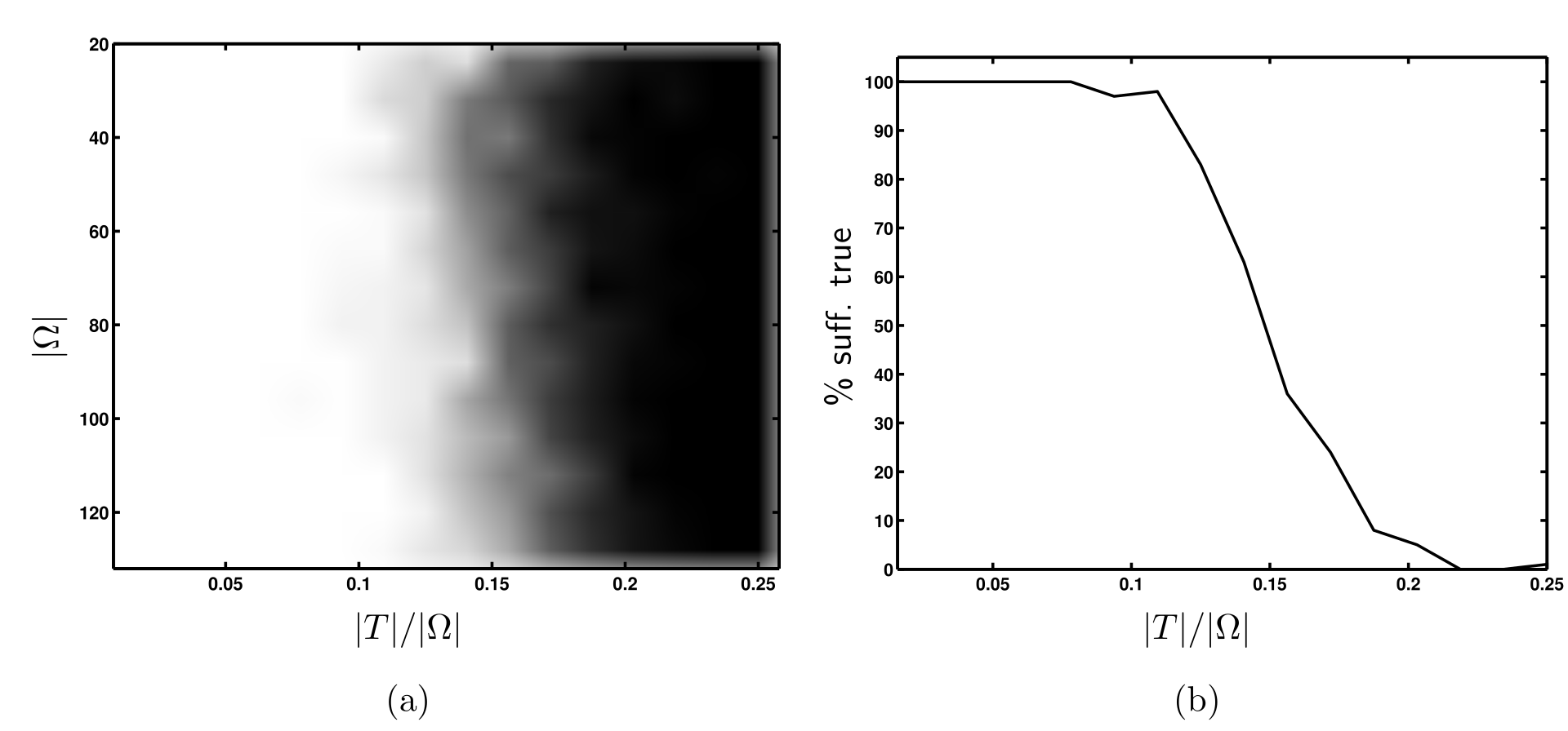
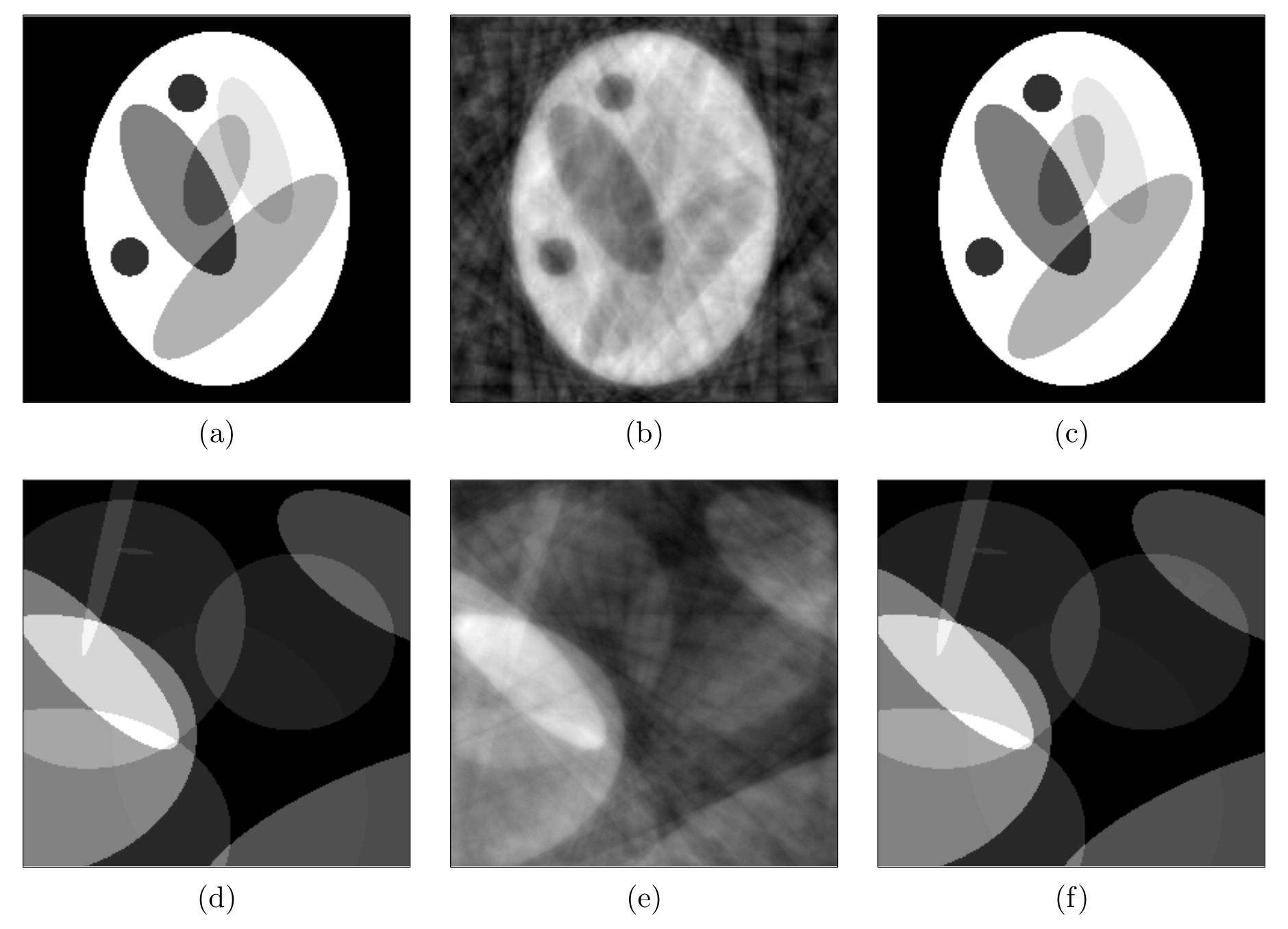
The experiment chooses a support and Fourier sample set uniformly without replacement, assigns random complex Gaussian amplitudes on the support, and solves the convex program. For N=512, each support/sample-size pair is tested 100 times. Figure 2 shows the empirical recovery map and its|Ω|=64cross-section; Figure 3 tests the specific certificate and has a different horizontal scale. The chosen certificate succeeds over a narrower region than the optimization itself, illustrating slack in that sufficient proof construction. Figure 4 retains both additional phantoms and all minimum-energy and TV reconstructions. Reported iteration counts and runtimes describe the authors’ implementation and historical hardware, not a current performance benchmark.
Figure 2: Recovery experiment for . (a) The image intensity
represents the percentage of the time solving recovered the
signal exactly as a function of (vertical axis) and
(horizontal axis); in white regions, the signal
is recovered approximately of the time, in black regions,
the signal is never recovered. For each pair,
experiments were run.
(b) Cross-section of the image in (a) at . We can see
that we have perfect recovery with very high probability for
. Figure 3: Sufficient condition test for . (a) The image
intensity represents the percentage of the time chosen as in
(2.11) meets the condition . (b) A
cross-section of the image in (a) at . Note that the
axes are scaled differently than in Figure 2. Figure 4: Two more phantom examples for the recovery problem discussed in Section 1.1. On the left is the original phantom ((d) was created by drawing ten ellipses at random), in the center is the minimum energy reconstruction, and on the right is the minimum total-variation reconstruction. The minimum total-variation reconstructions are exact.
6 Discussion
The discussion separates conditioning with a known support, reconstruction with noisy observations, and other synthesis/measurement pairs. Only the first is directly connected to a developed estimate in this manuscript; the others are described as preliminary or future work.
6.1 Stability
The same restricted Gram-matrix bound controls the condition of least-squares recovery when the support is known. A norm sufficiently below the diagonal scale keeps the inverse away from singularity. This supports local conditioning of that oracle problem under the stated sparsity and random-sampling regime. It is distinct from proving an error bound for the complete unknown-support convex recovery algorithm under arbitrary noise.
Equations
6.2 Robustness
With perturbed Fourier observations, exact recovery is no longer expected. The authors describe preliminary calculations suggesting small ℓ1 error for a small ℓ1 perturbation and explicitly defer detailed robustness results. The title’s terminology and this discussion therefore do not license a general noise-stability theorem beyond what the manuscript actually establishes.
Equation
6.3 Extensions
The proposed extension replaces the canonical/Fourier pair by other synthesis and measurement bases. Their incoherence would govern how many coefficients are required. The source reports this as work in progress and does not prove a uniform theorem for every pair of bases. Sparsity in one basis must be paired with a compatible measurement system.
7 Appendix
The appendix supplies the technical constant estimate for Theorem 3.3 and the scalar high-moment estimate used for the truncated certificate series. Both complete components invoked in the main proof; they are included here with all their original equations.
7.1 Proof of Theorem 3.3
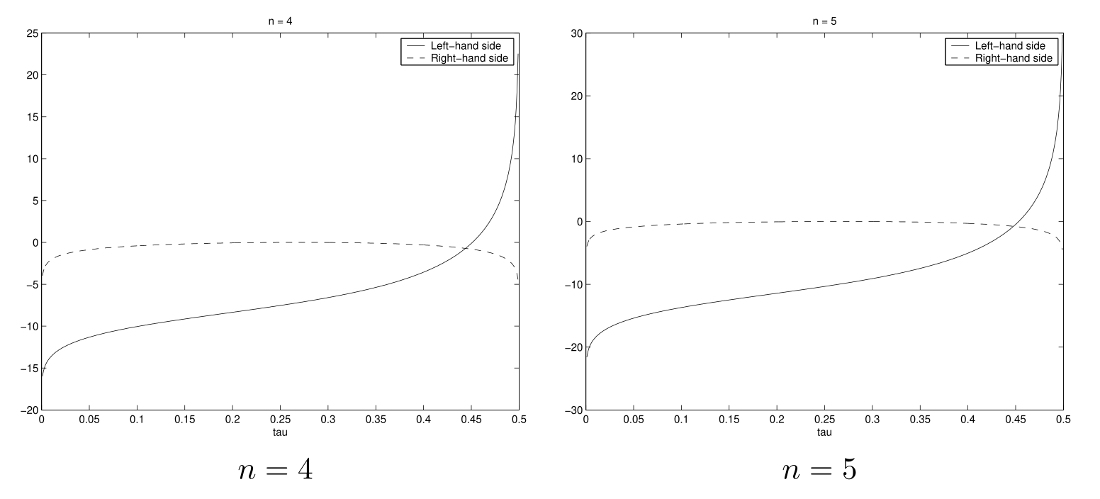
The proof reduces the technical comparison betweenan andbn to a scalar logarithmic inequality under τ≤0.44 and n≥4. Figure 5 plots its two sides for n=4 and 5. The source invokes simple numerical calculations for the stated constant range; the plot is an illustration, not independent proof for every parameter. Its original formulas and both plots are retained.
Equations 7.1
(7.1)
Figure 5: Behavior of the left and right-hand side of
(7.1) for two values of
7.2 Proof of Lemma 3.5
Expand a high even moment of a series term into multiple index paths, including the unit-modulus signal phases. Group repeated frequencies and apply the same partition identity as in Section 4. Because the starting point is fixed, the count has one fewer free signal index than the trace calculation, producing the additional support-size factor in Lemma 3.5. The final estimate parallels the matrix-moment argument while preserving that distinction.
Equations 7.2–7.4
(7.2)
(7.3)
(7.4)
23 references
[1] S. Boucheron, G. Lugosi, and P. Massart, A
sharp concentration inequality with applications, Random
Structures Algorithms16 (2000), 277–292.
[4] A. H. Delaney, and Y. Bresler, A fast and
accurate iterative reconstruction algorithm for parallel-beam
tomography, IEEE Trans. Image Processing, 5 (1996),
740–753.
[8] D. L. Donoho and M. Elad, Optimally sparse
representation in general (nonorthogonal) dictionaries via
minimization. Proc. Natl. Acad. Sci. USA100 (2003),
2197–2202.
[9] M. Elad and A.M. Bruckstein, A generalized
uncertainty principle and sparse representation in pairs of
bases, IEEE Transactions on Information Theory, 48
(2002), 2558–2567.
[10] P. Feng, and Y. Bresler, Spectrum-blind
minimum-rate sampling and reconstruction of multiband signals, in
Proc. IEEE int. Conf. Acoust. Speech and Sig. Proc.,
(Atlanta, GA), 3 (1996), 1689–1692.
[11] P. Feng, and Y. Bresler, A multicoset sampling
approach to the missing cone problem in computer aided tomography,
in Proc. IEEE Int. Symposium Circuits and Systems, (Atlanta,
GA), 2 (1996), 734–737.
[12] A. Feuer and A. Nemirovsky, On sparse
representations in pairs of bases, Accepted to the IEEE
Transactions on Information Theory in November 2002.
[20] J. A. Tropp, Just relax: Convex programming
methods for subset selection and sparse approximation, Technical
Report, The University of Texas at Austin, 2004.
[21] M. Vetterli, P. Marziliano, and T. Blu,
Sampling signals with finite rate of innovation, IEEE
Transactions on Signal Processing, 50 (2002),
1417–1428.
[22] A. C. Gilbert, S. Guha, P. Indyk, S.
Muthukrishnan, M. Strauss, Near-optimal sparse Fourier
representations via sampling, 34th ACM Symposium on Theory of
Computing, Montréal, May 2002.
[23] A. C. Gilbert, S. Muthukrishnan, and M.
Strauss, Beating the bottleneck in estimating -term Fourier
representations, unpublished manuscript, May 2004.