At a glance
Simulation Affordance Grids (SAGrid) predicts where a simulator should place toggle buttons, heat sources and water sources on an unlabeled mesh. It combines pretrained TRELLIS geometry and DINOv2 semantics, then learns a dense distance-to-affordance field from a small annotated object set.
On the held-out sink/stove validation set, mean localization error is about 4.8 cm. Automatically annotated Objaverse-XL assets improve some downstream policy results, reaching 49% steak-cooking and 24% cup-filling success. These are two simulated tasks with objects initially grasped, rather than demonstrations of complete household skills or real-world transfer.
Introduction
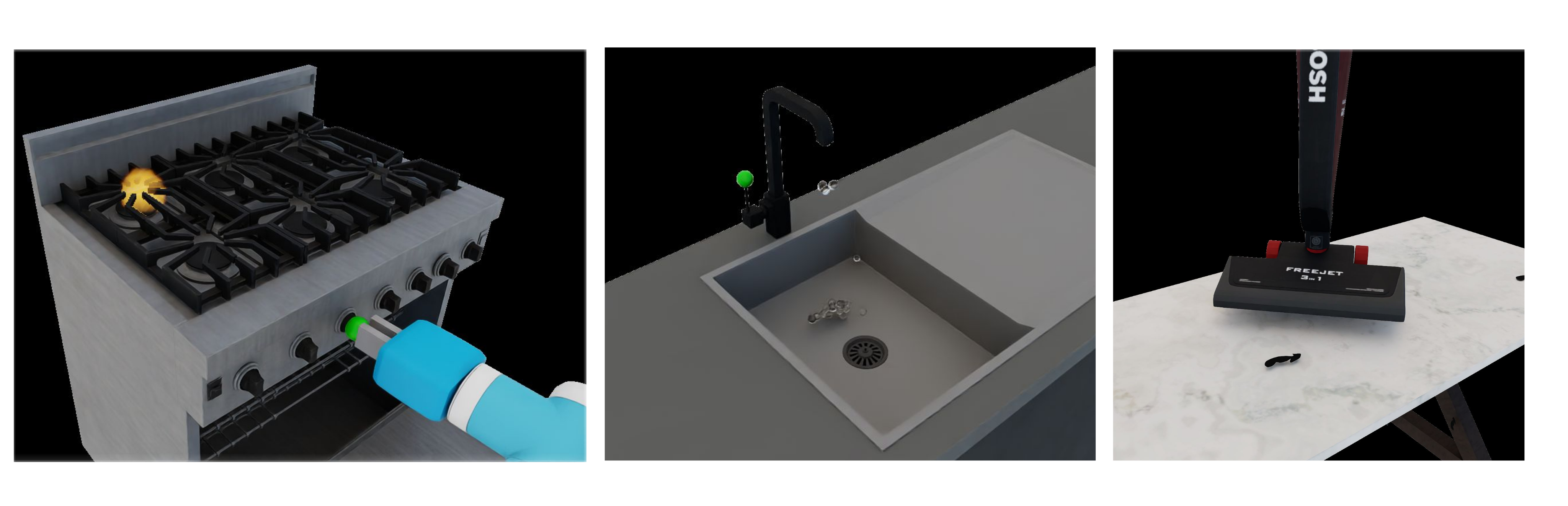
Many household simulators need annotations that rigid-body geometry alone cannot supply: where water should emerge, a burner should heat, or a switch should activate a device. Figure 1 illustrates these simulation-specific affordances [1] [3].
The scaling problem therefore concerns functional annotations as well as mesh count and rollout volume. SAGrid expands the available assets without manually annotating each new mesh, although it still depends on annotated training objects and substantial pretrained representations.
Simulation Affordance Grids
The input is a textured mesh; the output is a set of positions and affordance labels. A separate predictor is trained for each label/category combination used in the experiments. A predicted heat source, for example, identifies a point where the simulator should emit heat.
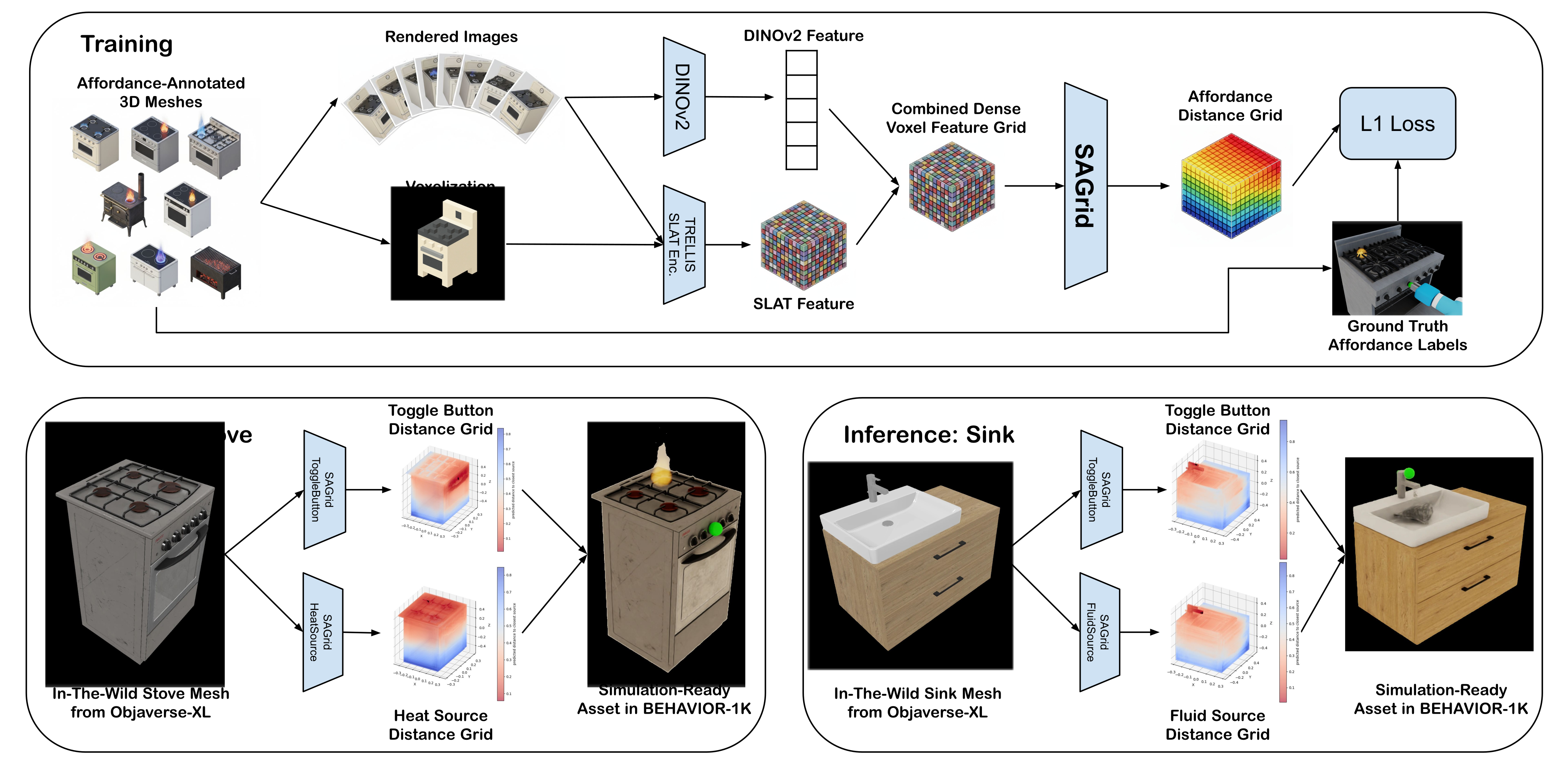
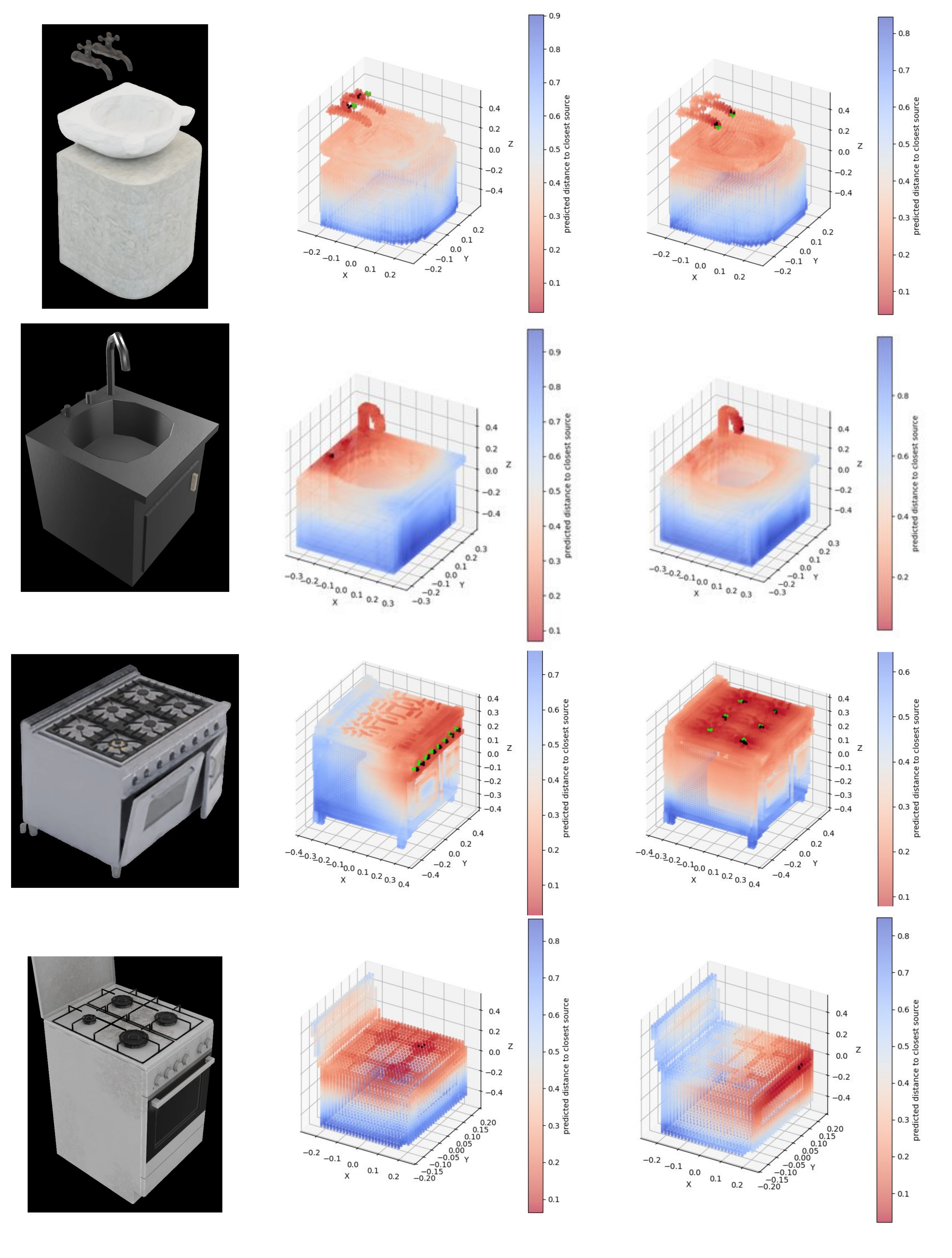
The complete Figure 2 retains both the feature/training pipeline and the stove/sink inference examples. The method predicts annotations, rather than simulating hidden physical mechanisms such as actual plumbing.
Architecture
The dense 64³ input grid has 1,033 channels per voxel: eight TRELLIS structural-latent features, a 1,024-dimensional DINOv2 object vector broadcast across the grid, and one occupancy mask. The global vector aggregates 150 rendered views [4] [5].
A 3D CNN with batch normalization and ReLU predicts one distance value per voxel through a 1×1×1 head and Softplus. The small labeled set should be distinguished from total learning and preprocessing cost: the backbone pretraining and 150-view feature extraction are additional inputs to the system.
Feature extraction
Meshes are rendered from 150 random views, encoded with DINOv2, normalized into a unit bounding box, voxelized, and passed through the pretrained TRELLIS encoder. The pipeline combines structural latents, semantic features and occupancy into a dense grid.
This representation assumes access to the 3D mesh and its renderings. Its results do not directly establish performance from a single noisy camera image or an incomplete real-world reconstruction.
Training
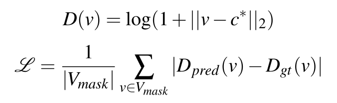
The network regresses log(1+distance) to the nearest labeled affordance. An L 1 objective averages the absolute error over occupied voxels; the complete target and loss formulas are retained. Training uses AdamW, a cosine learning-rate schedule, translations, right-angle rotations, reflections and warping.
Four predictors are used: stove heat source, stove toggle button, sink fluid source and sink toggle button. The source reports 31 annotated sinks and 14 stoves, with five of each held out, implying 26 training sinks and nine training stoves. Its “as few as 10 objects” phrasing is approximate, rather than the literal stove split described later.
Equation
Inference
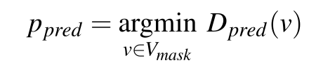
DINOv2 cosine similarity first filters candidate meshes. The feature pipeline and learned field then locate the occupied voxel with the smallest predicted distance. That position is mapped back to object coordinates and projected onto the collision mesh. VLM-predicted masses and CoACD collision geometry are additional asset-processing steps [21] [22] [23].
Known multiple instances can be extracted with thresholding and k-means, but the demonstrated pipeline selects one instance per type. Unknown instance counts require a further counting mechanism. The intro’s mention of multilateration should not replace the concrete minimum-selection procedure specified here.
Equation
Experimental setup
BEHAVIOR-1K supplies annotated sinks and stoves, the simulation environment and the held-out validation objects. New meshes come from the Sketchfab subset of Objaverse-XL. Affordance localization and policy success are separate evaluations.
The five-per-category holdout is small, and reported results do not include seed uncertainty or confidence intervals. Quantitative policy testing remains on held-out BEHAVIOR-1K objects; the Objaverse examples show the asset-expansion process, rather than a separately reported broad labeled-mesh test benchmark.
Architecture comparison
CNN-1 achieves 4.84 cm mean localization error, compared with 6.59 cm for CNN-2,7.13 cm for PointNet and 12.87 cm for the MLP. The complete architecture table retains every kernel, padding, channel and dilation specification [24].
The comparison does not isolate receptive field as the sole cause: CNN-1 and CNN-3 use the same listed kernel/dilation pattern but different channel widths. Projecting predictions to the mesh reportedly reduces surface-normal error, but the paper provides no separate post-projection numerical table. Figure 3 shows representative fields and locations.
| Model ID | CNN Architecture | Error (cm) |
|---|---|---|
| CNN - 1 | [3,1,1024],[3,4,512,4],[3,1,256],[3,1,128] | 4.84 |
| CNN - 2 | [3,1,32],[3,1,16] | 6.59 |
| CNN - 3 | [3,1,128],[3,4,64,4],[3,1,32],[3,1,16] | 6.78 |
| PointNet | Point cloud architecture | 7.13 |
| CNN - 4 | [3,1,256],[3,4,128,4],[3,1,64],[3,1,32] | 7.25 |
| CNN - 5 | [3,2,32,2],[3,1,16] | 10.29 |
| CNN - 6 | [3,1,32],[3,2,16,2] | 11.47 |
| MLP | [512], [256], [128] | 12.87 |
Affordance prediction baselines
TableII retains all retrieval, VLM triangulation and generated-marker baselines, both RANSAC variants and every per-affordance error. SAGrid’s mean error is 0.048 m, versus 0.1654 m for cosine embedding search and 0.1285 m for the best listed Gemini triangulation configuration.
Ray RANSAC aggregates view rays; point RANSAC aggregates ray-cast 3D points. These are evaluated on the same small holdout, while their pretrained models, inference procedures and computational budgets differ. No uncertainty or matched-cost comparison is reported.
The text names Qwen3-VL 8B, but reference 25 is the general Qwen3 technical report. The source does not provide a dedicated VL-version citation or enough API/version detail to infer a fully fixed baseline implementation [25].
| Model | Method | toggle sink | fluid source | toggle stove | heat source | Avg |
|---|---|---|---|---|---|---|
| Embedding Search | ||||||
| DINOv2+TRELLIS | cosine | 0.0766 | 0.1012 | 0.1959 | 0.2881 | 0.1654 |
| DINOv2+TRELLIS | L2 | 0.1013 | 0.1046 | 0.2100 | 0.2607 | 0.1691 |
| VLM Triangulation | ||||||
| Gemini 2.5 Flash | ray-ransac | 0.1057 | 0.1192 | 0.1428 | 0.1462 | 0.1285 |
| Gemini 2.5 Flash | point-ransac | 0.1354 | 0.1621 | 0.1959 | 0.1731 | 0.1666 |
| Qwen3-VL 8B | ray-ransac | 0.2196 | 0.2559 | 0.2070 | 0.2613 | 0.2360 |
| Qwen3-VL 8B | point-ransac | 0.4391 | 0.5067 | 0.1295 | 0.2695 | 0.3362 |
| Image Generation | ||||||
| NanoBanana 2.5 | ray-ransac | 0.2219 | 0.2040 | 0.2838 | 0.2147 | 0.2311 |
| NanoBanana 2.5 | point-ransac | 0.3788 | 0.3818 | 0.3042 | 0.1607 | 0.3064 |
| SAGrid (Ours) | ||||||
| CNN-1 | distance field | 0.038 | 0.033 | 0.057 | 0.064 | 0.048 |
Robot policy learning
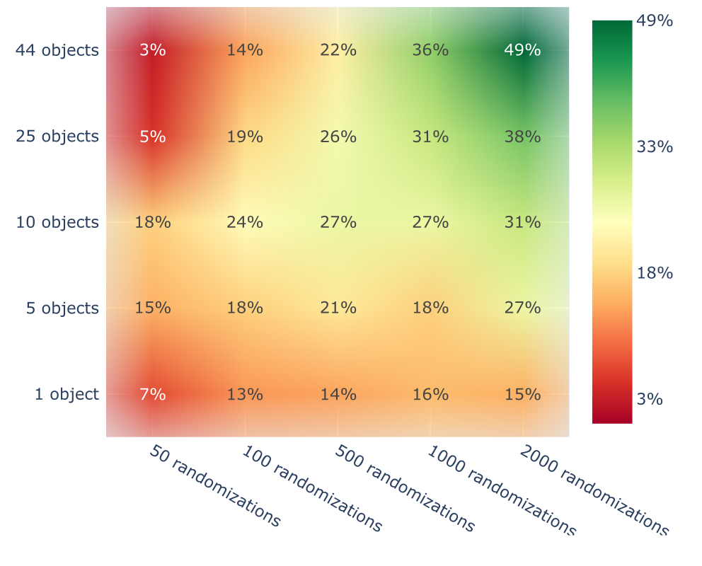
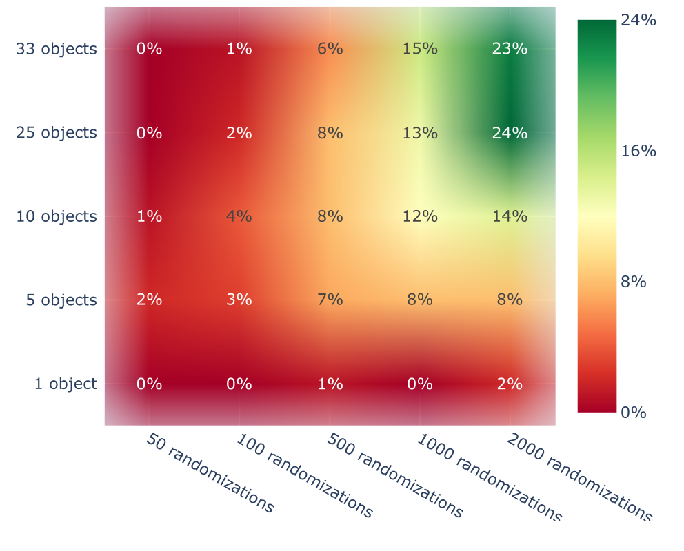
Each task has a 5×5 grid of Diffusion Policy experiments: one to the maximum number of objects, crossed with 50 to 2,000 demonstrations. Demonstrations use heuristic waypoints and motion planning from randomized configurations; trajectories are spread across objects. Each policy trains for 10,000 steps and is evaluated on 100 randomized rollouts [26] [27].
Episodes begin with the manipulated object already grasped. The source says the first 10 objects are original BEHAVIOR-1K assets, but its earlier stove split leaves only nine non-held-out stoves. That count discrepancy is unresolved; the paper does not provide enough asset-ID detail to establish which explanation is correct.
Cooking steak
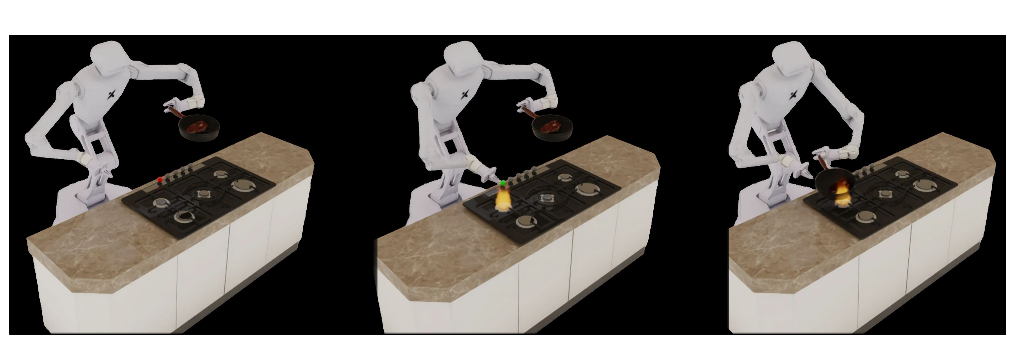
The policy activates a burner and places the held pan/steak over its heat source. With 2,000 demonstrations, 44 objects yield 49% success versus 31% with 10 objects. A single object reaches 15–16% at the two largest demonstration budgets.
Diversity is not uniformly beneficial: at 50 demonstrations, 44 objects score 3%, versus 18% for 10 objects. Even at 500 demonstrations, 10 objects score 27% and 44 objects 22%. The benefit depends on sufficient examples per object; the grid supports an interaction between diversity and data volume rather than a monotonic diversity rule.
Cup filling
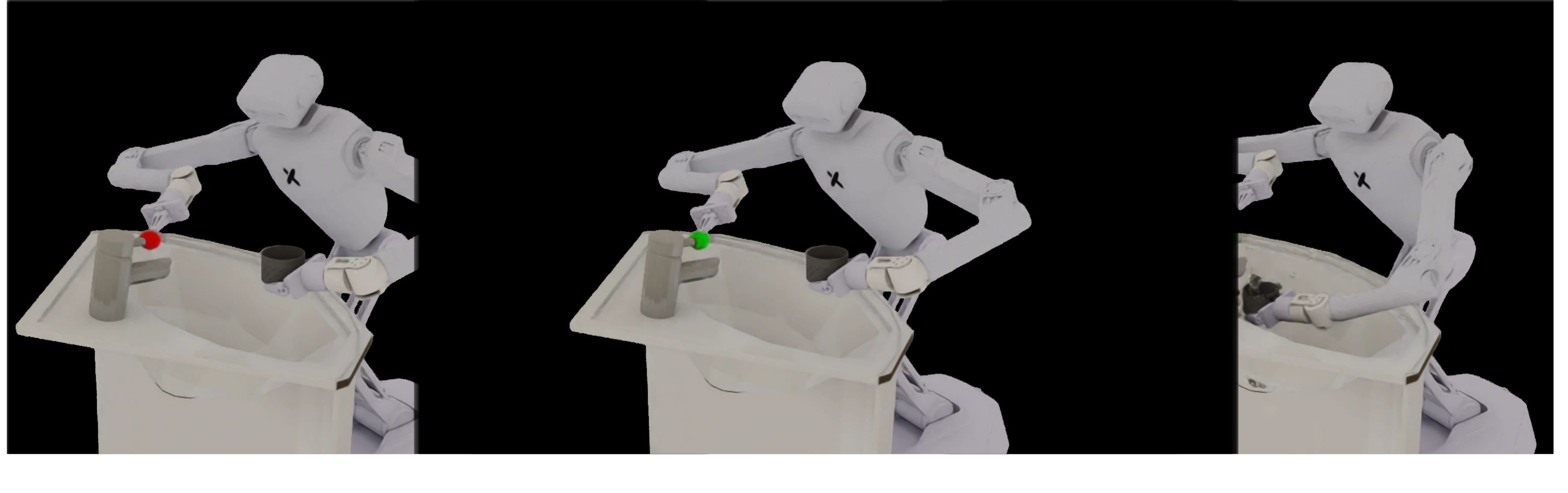
The dual-arm policy activates a faucet and places the held cup beneath its fluid source. At 2,000 demonstrations, 25 training sinks reach 24% success, 33 sinks 23%, 10 sinks 14% and one sink 2%.
The claimed diversity–annotation-noise tradeoff at 33 objects is an interpretation of a one-point difference, without repeated-seed uncertainty or a controlled annotation-noise experiment. Most evaluation attempts still fail, so the result supports a useful asset-expansion direction rather than task reliability.
Limitations
The demonstrated affordances are dimensionless, orientationless points. Volumes, spray cones and other parameterized shapes with a full pose remain future work. The displayed vacuum-cleaner example motivates the problem; it is not an additional evaluated affordance category.
Only one affordance instance per type is extracted in the experiments. Robustly recovering unknown counts is proposed future work. The results cover two object categories and two simulated tasks; broad category transfer, real-robot performance, pipeline throughput and deployment cost are not established.
Conclusion
Automatically locating functional simulation points can make previously unusable meshes available for data collection. The paper’s main evidence is a small localization study and controlled diversity/data grids in two tasks.
Its practical contribution is separating simulation-affordance annotation from manual asset preparation. Stronger claims about generalization, reliability or removal of all human preparation work need broader evaluation and a fuller accounting of the preprocessing pipeline.
Acknowledgments and resources
Figure 2 artwork was created with assistance from AI models, as stated in the paper. The work acknowledges the AI2050 program at Schmidt Sciences.
The authors’ repository provides the original paper, code, figures, configurations and inference documentation. The reading edition follows the complete seven-page author PDF.