Introduction · Extension constants
Intuition. Imagine a calibration function defined only at measured inputs. A Lipschitz condition says nearby inputs cannot produce wildly different outputs: the output distance is at most a fixed multiple of the input distance. The paper asks how much that multiplier must increase when the function is extended to unmeasured inputs.
Reading the math. Hilbert space generalizes Euclidean vector geometry, retaining an inner product for lengths and angles. A key tool replaces n high-dimensional points with shorter vectors while approximately preserving every pairwise distance. The required dimension grows logarithmically with n, with extra dimensions for tighter accuracy. This finite-set guarantee is not a neural-network storage-capacity formula.
The problem is to extend a Lipschitz map from n points in an arbitrary metric space to the whole space when the target is Hilbert space. L(X,n) measures the worst multiplicative increase in Lipschitz constant. Kirszbraun’s theorem gives constant one for Hilbert domains; general domains can force growth.
The main theorem bounds that cost by a universal constant times the square root of log n. Finite-set dimension reduction is its main tool. The paper also proves lower bounds, studies separated-domain extensions, poses historical questions, and includes an appendix credited to Yoav Benyamini. Its scope is broader than the familiar dimension-reduction lemma.



Introduction · Notation and comparison bounds
The authors use Log x for the maximum of one and the natural logarithm. Balls, unit spheres, the uniform norm of a bounded function, and Banach–Mazur distance are defined before the main argument.
For 1≤p<2, the proposed sharp extension growth remains unresolved in this paper. Its lower bound includes a log log n denominator, whereas the comparison upper bound has the corresponding power of log n alone. Those directions and exponents matter when comparing the theorems.




1 · Lemma 1: finite Euclidean dimension reduction
For a fixed distortion tolerance, an n-point Euclidean set maps to dimension at most a tolerance-dependent constant times log n while controlling every pairwise distance through the displayed two-sided Lipschitz bound. The original ambient dimension disappears from the final bound.
The proof samples a rank-k projection by conjugating a coordinate projection with a Haar-random orthogonal matrix. Concentration on the sphere controls each normalized difference vector; a union bound controls all pairs. It proves existence of a suitable finite-set map, rather than success for every projection or arbitrary learned representation.







1 · Concentration, scale and logarithmic dimension
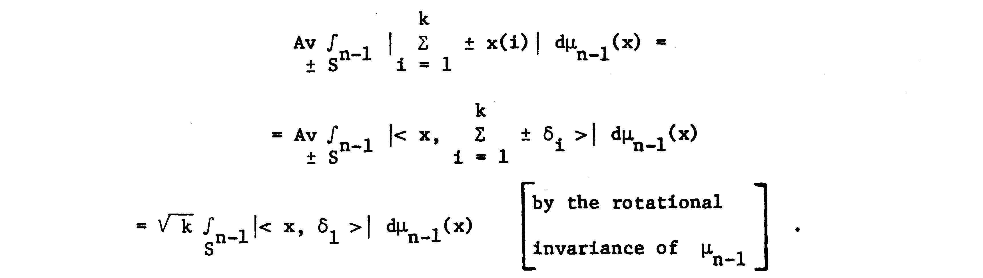
A scaled projection seminorm concentrates around its median. The proof relates median and mean, then estimates the mean with rotational invariance and Khintchine’s inequality. Its typical scale is the square root of k, turning an additive concentration window into relative distortion.
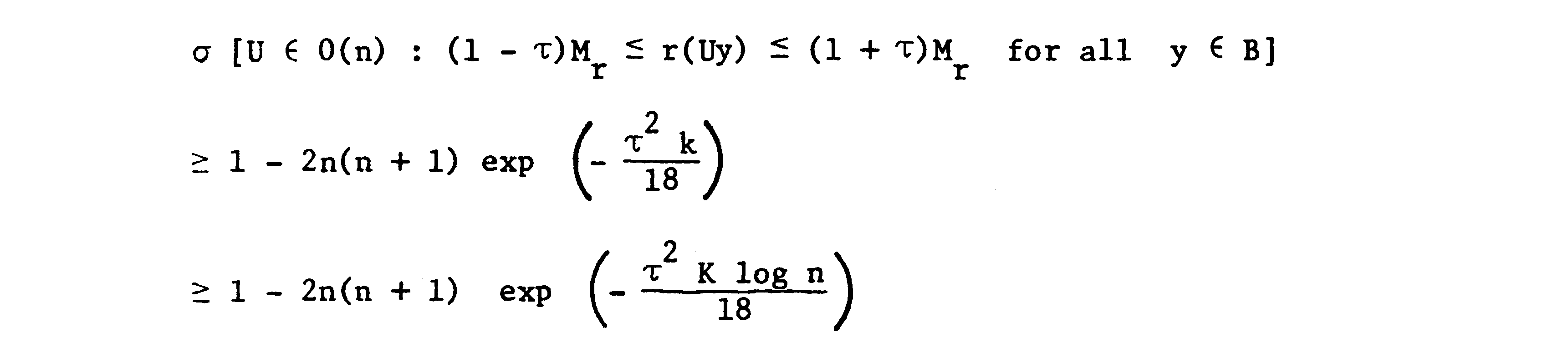
Taking k proportional to the tolerance-dependent log n makes the failure bound less than one. A packing argument then shows logarithmic dimension is necessary for fixed sufficiently small distortion: a bounded k-dimensional ball cannot contain arbitrarily many separated images of an orthonormal set. This does not itself establish exponential storage of independently readable semantic concepts in a neural model.
Equations PDF p.4 · display 15–PDF p.5 · display 30














1 · Theorem 1: extending into Hilbert space
Dimension reduction first places the n image points in a controlled k-dimensional Euclidean configuration. Coordinatewise extension through an infinity-norm space handles the arbitrary metric domain; comparison of finite-dimensional norms costs a square root of k. Kirszbraun’s theorem controls reconstruction into the Hilbert target.
Combining these steps gives the square-root-of-log-n extension bound. The construction extends a specified finite map; it does not assert a low-dimensional linear extension on the whole original ambient space.









1 · Theorem 2: separated domains
A domain subset with minimum separation ε and finite diameter D admits an extension with cost bounded by 6 D/ε. The proof factors the map through a coordinate-indexed sequence space, uses a weak Grothendieck inequality, and extends an infinity-norm-valued map coordinatewise.
This limits a lower-bound strategy using coarse nets of a sphere. A coarse separated net already admits a controlled extension, so a hard linear projection problem cannot automatically be recovered from every coarse nonlinear approximation.











1 · Lemmas 2–4: tools for the lower bound
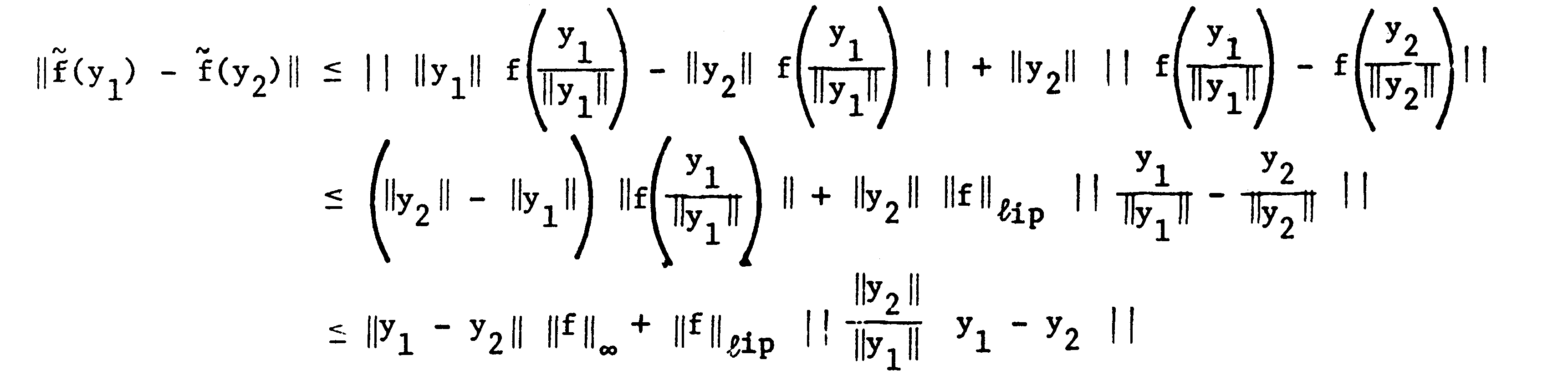
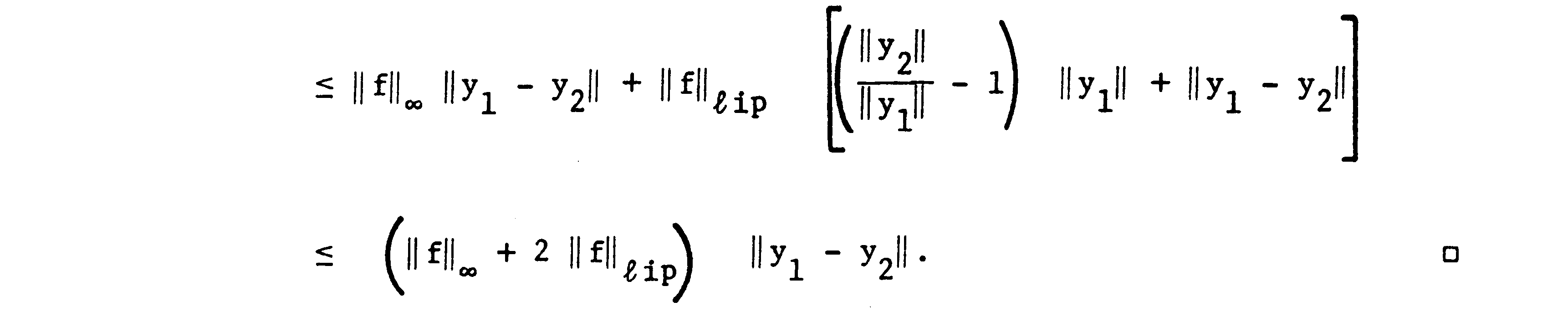
Lemma 2 extends a sphere map by positive homogeneity, controlling its Lipschitz constant through its sphere Lipschitz and uniform norms. Lemma 3 obtains an ε-net of cardinality at most the displayed exponential function of dimension by comparing volumes of disjoint small balls.
Lemma 4 supplies nearly Euclidean finite-dimensional subspaces of Lp,1≤p<2, that have large projection constants. They furnish an obstruction: turning an accurate nonlinear extension into a low-norm linear projection would contradict that lower bound.
Equations PDF p.8 · display 51–PDF p.10 · display 64












1 · Proposition 1: linearizing a Lipschitz approximation
The proposition converts a Lipschitz approximation to a bounded linear operator on a subspace into an operator between dual spaces with controlled norm and restriction error. For a reflexive target, an adjoint gives a map back into the original target.
The proof uses norm-one projections from scalar Lipschitz-function spaces onto ordinary dual spaces and their compatibility with restriction. This connects the nonlinear extension problem to linear projection obstructions; pointwise approximation alone would not give that connection.








1 · Lemma 5: smoothing a homogeneous map
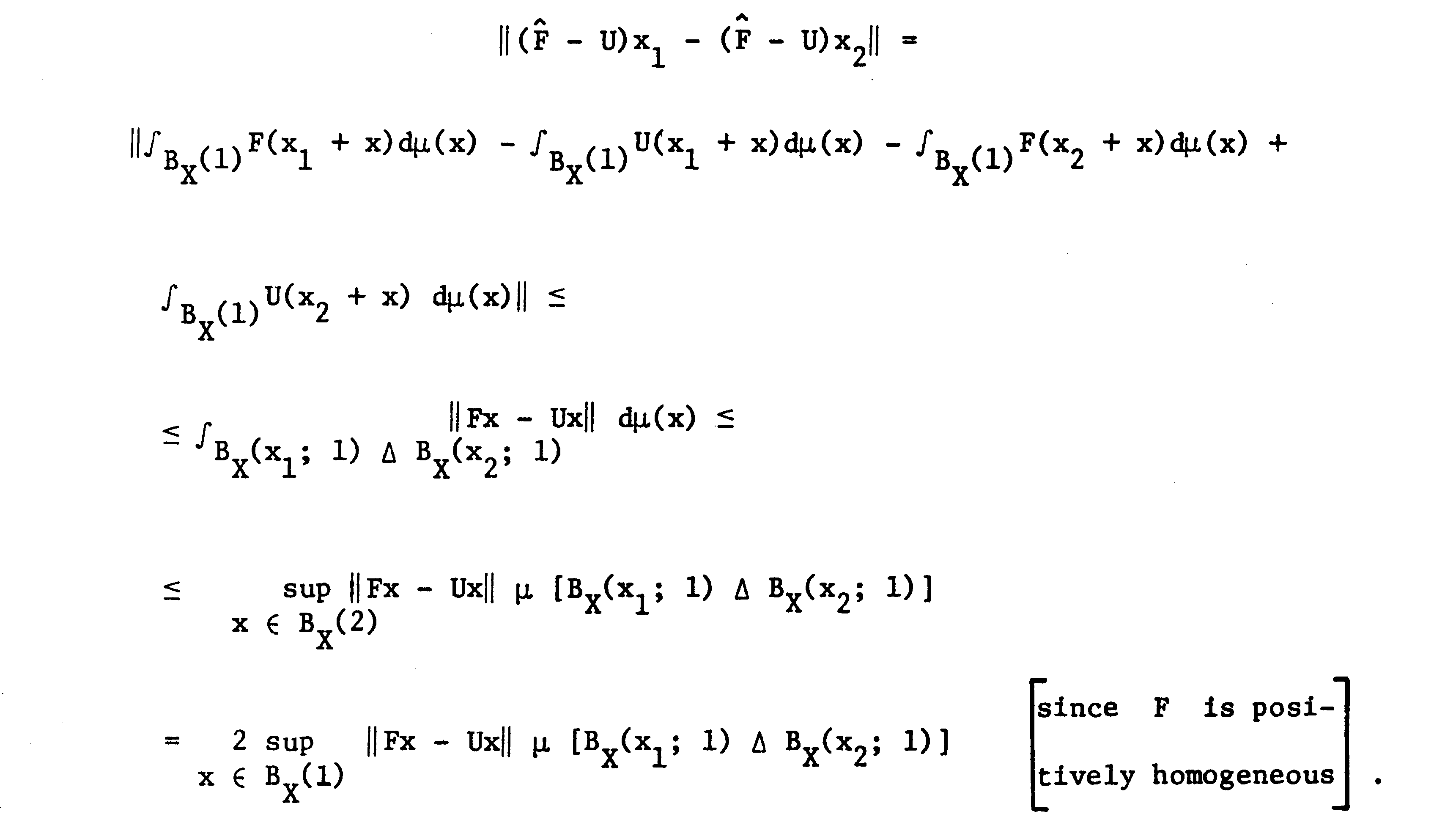
Averaging a homogeneous Lipschitz map over the unit ball of a finite-dimensional subspace controls its regularity on that subspace. Comparing overlaps of translated balls turns uniform approximation on a sphere into Lipschitz approximation.
The estimates retain dimension factors and constants. A final homogeneous extension gives a globally defined controlled map. This supplies the regularity needed before Proposition 1 can be used in the lower-bound argument.
Equations PDF p.11 · display 73–PDF p.13 · display 84











1 · Theorem 3: the Lp lower bound
For 1≤p<2, the extension cost is at least an absolute constant times (log n/log log n) raised to 1/p−1/2. The proof chooses a nearly Euclidean subspace with a large projection constant, takes a sufficiently fine finite net, extends its identity map, then homogenizes, smooths and linearizes.
The net must be fine enough that the resulting linear approximation yields an actual projection. Balancing that accuracy requirement with net cardinality produces the log log n term. The gap to the upper bound remains explicit in this 1984 article.










2 · Four open problems posed in 1984
The questions concern sharp extension growth, nonlinear analogues of linear Lp extension results on either side of p=2, dimension reduction beyond Hilbert spaces, and controlled Hilbert embeddings of arbitrary finite metric spaces. These are recorded as historical questions; no claim is made that they all remain open today.
The final question proposes square-root-of-log-n distortion. A preceding proposed finite-dimensional Banach embedding would imply it, and a cube inequality motivates sharpness if the asserted embedding exists. These conjectural directions are separate from the consequences already proved by Lemma 1.






3 · Benyamini’s appendix: the retraction lemma
The appendix replaces the Hilbert target in the separated-domain theorem by any Banach space. It builds a controlled retraction from an infinity-norm space onto the positive part of an ℓ1 unit ball, then a controlled map onto its coordinate segments.
A threshold subtracts the same scalar from positive coordinates until the remaining ℓ1 mass is at most one. A second threshold leaves at most one active coordinate. The displayed formulas prove Lipschitz bounds and fix coordinate basis vectors. Benyamini’s contribution is explicitly credited.










3 · Completing the Banach-target extension
Map the separated set to coordinate basis vectors, assigning one point to zero, and extend that map coordinatewise in an infinity-norm space. Extend the target-valued map linearly along the coordinate segments and compose with the appendix’s controlled segment map.
The resulting 4 D/ε bound does not require Hilbert structure in the target. The edition follows the full 18-page article, including proofs, appendix and fourteen references. It preserves standalone mathematical displays from the original scan at native pixel resolution, excludes download footers, and condenses source prose rather than reproducing full text columns.






