Overview
Virtual weights can look strong while doing little useful computation. This report separates their effects on predictions from their effects on predictive loss.
Authors
Nicholas L. Turner, Jeffrey Wu, and Joshua Batson.
Affiliations
Anthropic.
Published
Published August 21, 2026.
Introduction
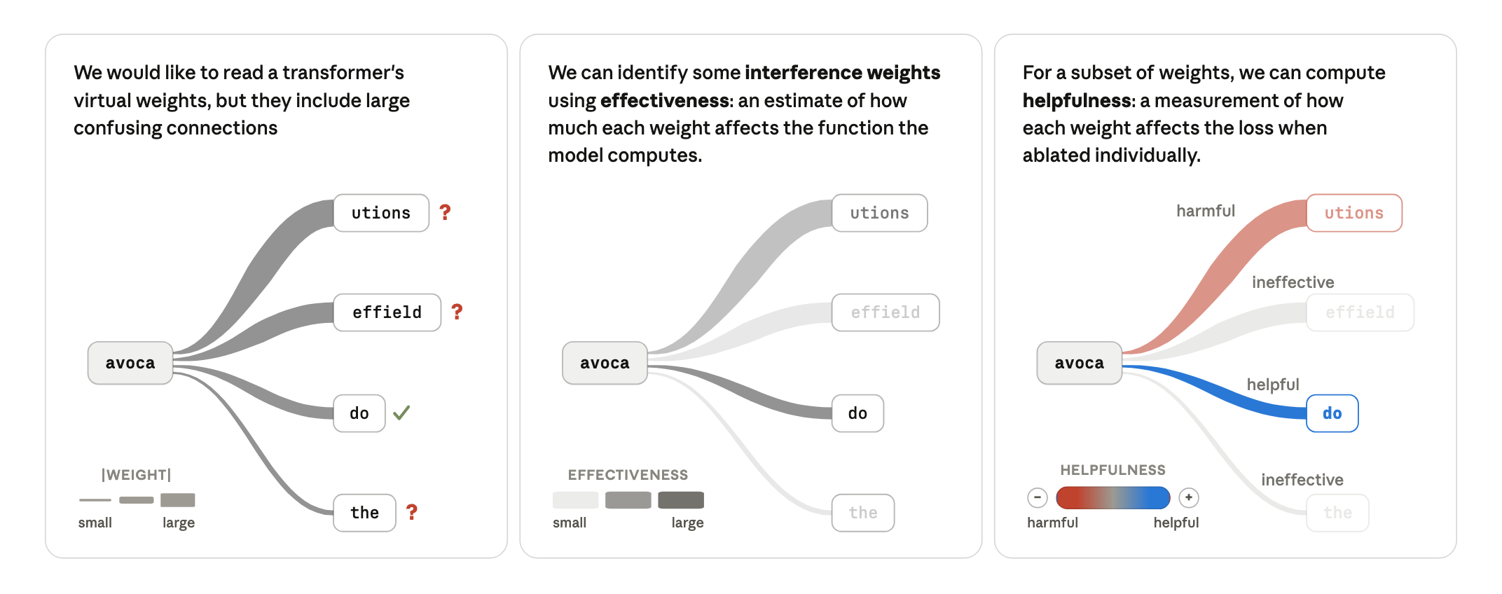
Superposition forces interpretable features to interact through a narrow residual stream, creating interference weights that are irrelevant or harmful on the data distribution. Expanding a trained one-layer transformer into virtual weights makes this concrete: a large connection from “IN” to “utions” always hurts, since that continuation never occurs in training. Earlier toy-model work motivated this test. Two measurements matter: effectiveness estimates how much a weight changes the output distribution; helpfulness measures whether ablating it raises or lowers loss. Removing the least effective 70% costs about 0.01 nats, but the surviving model remains much larger than the original. The analysis builds on the circuit-tracing replacement model.
A motivating example
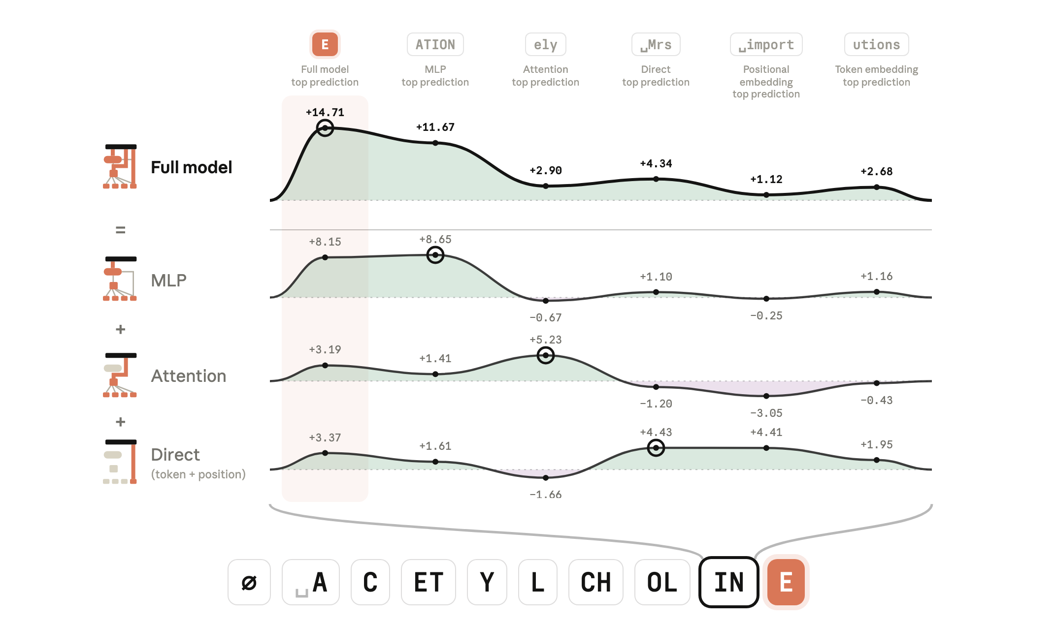
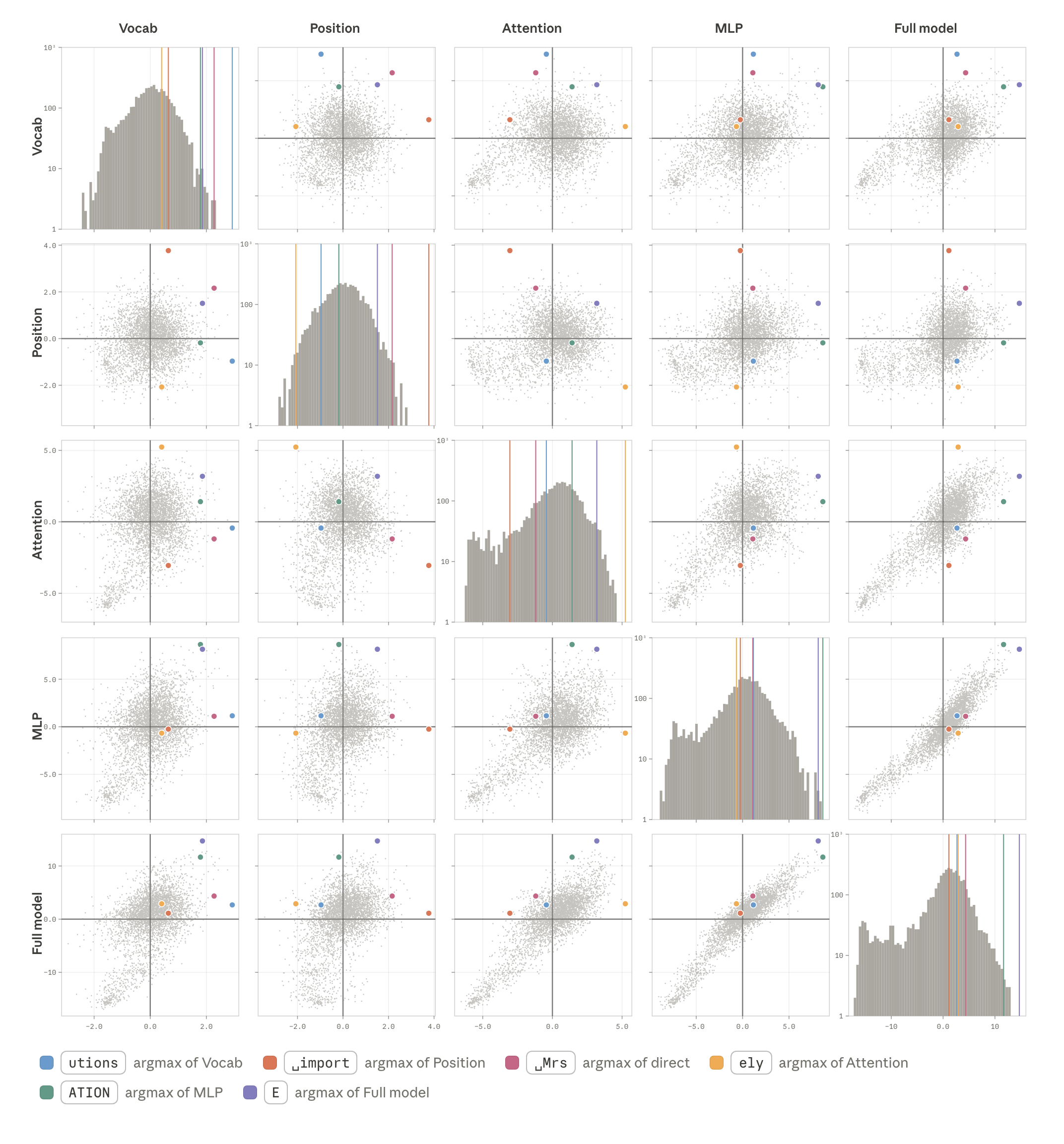
When completing “ACETYLCHOLINE”, direct, attention, and MLP paths each favor a different wrong continuation. “E” wins because all three support it moderately. Large individual votes therefore need not be useful circuits; loss interventions distinguish helpful competition from tolerated noise.
The virtual weight model
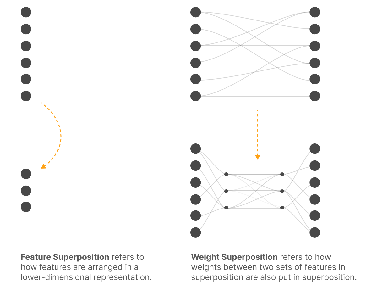
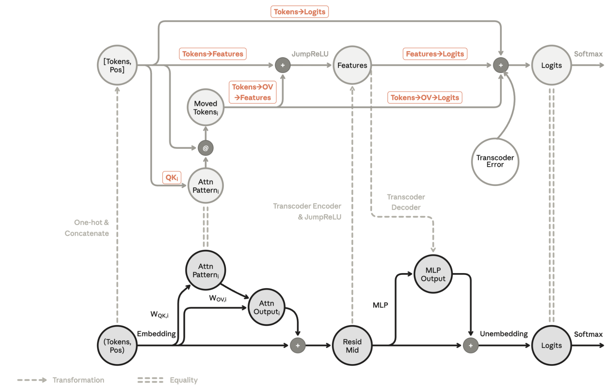
Replace the MLP with a 4,096-feature transcoder and expand six matrix-product families connecting tokens, positions, features, and logits. The original normalization-free transformer has width 256, vocabulary 4,096, and 1,024 positions. Its virtual-weight representation grows from 2.9 million parameters to roughly 331 million, while an explicit transcoder-error correction preserves the original forward pass. QK interactions determine attention; the other five families are linear maps conditioned on their inputs.
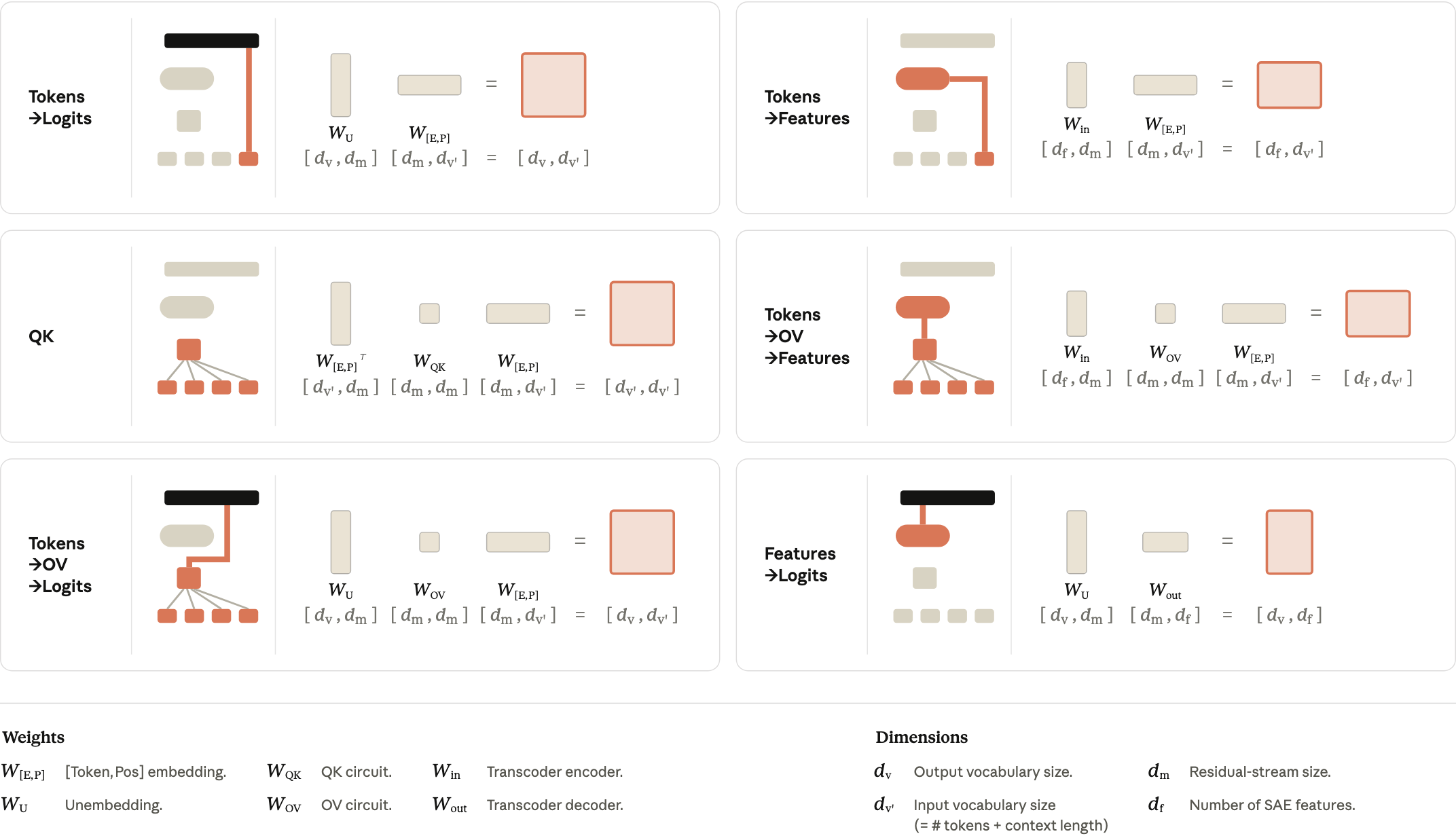
Effectiveness and helpfulness
Fisher effectiveness is a second-order estimate of the output KL divergence caused by ablating a weight, averaged over about 537 million token presentations. Helpfulness is the average increase in actual loss under ablation; positive means useful, negative means harmful. The latter requires many samples and is expensive for internal paths, so selected weights are evaluated over the training set or one billion token presentations with 95% confidence intervals. Effectiveness improves earlier coactivation proxies but does not determine helpfulness’s sign.
Equation
Effectiveness surfaces helpful weights but does not isolate them
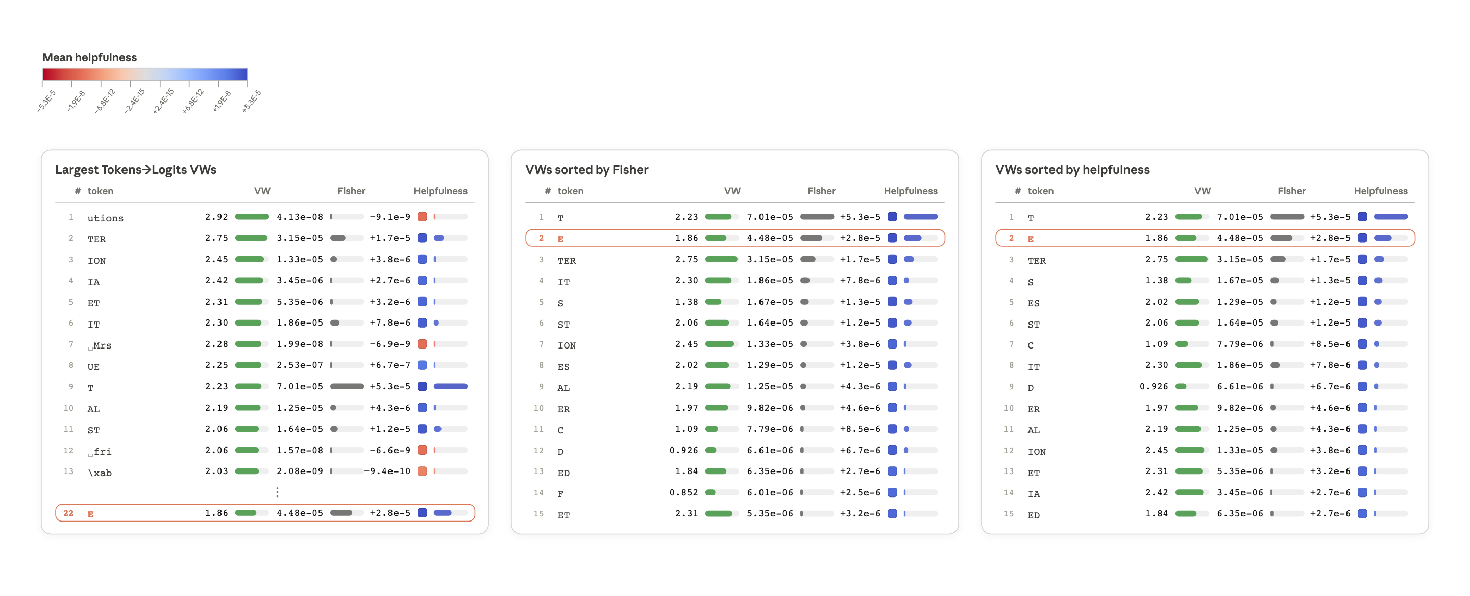
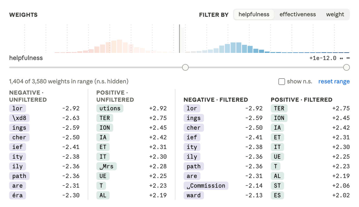
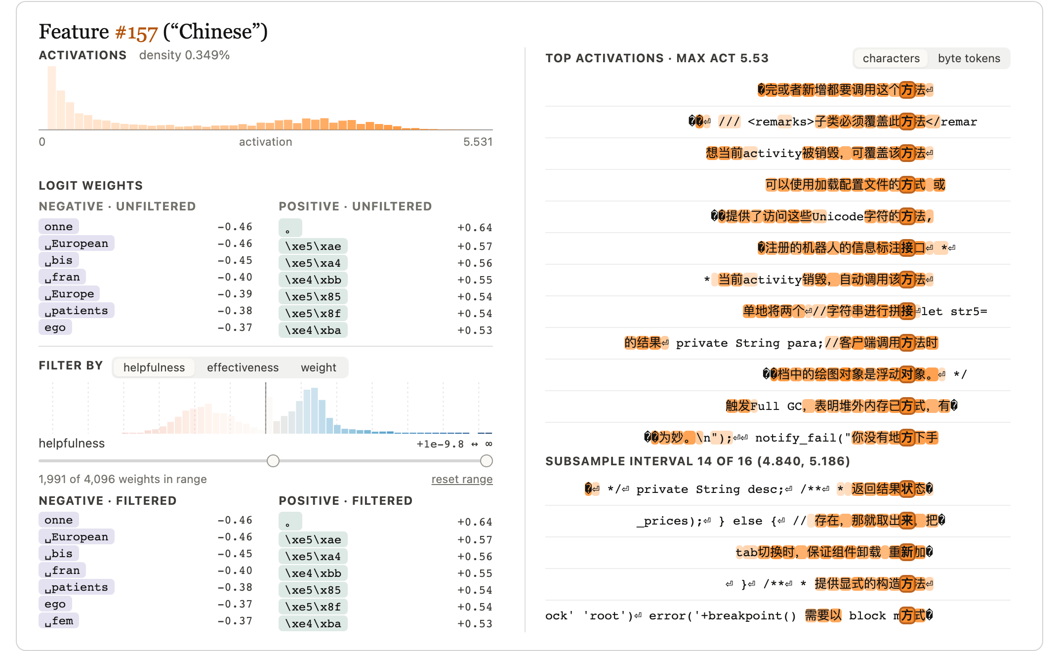
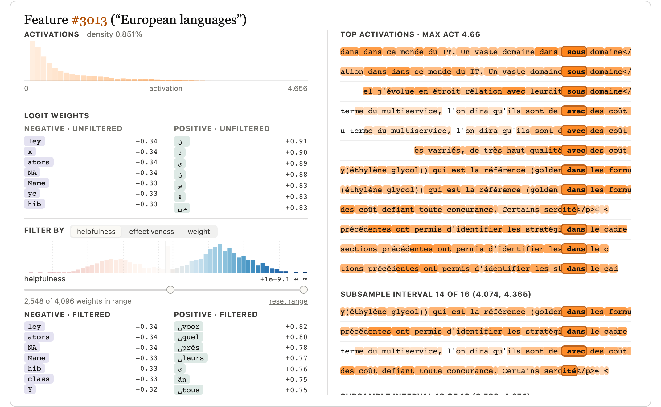
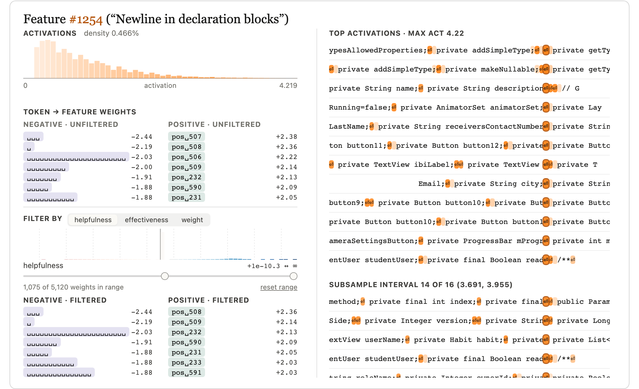
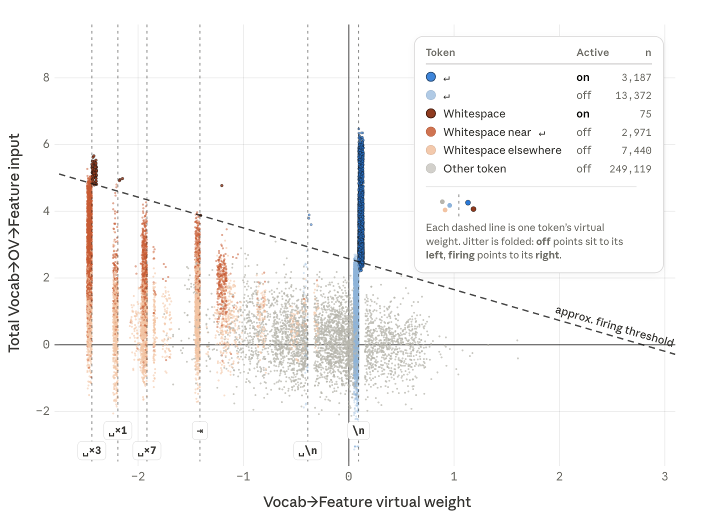
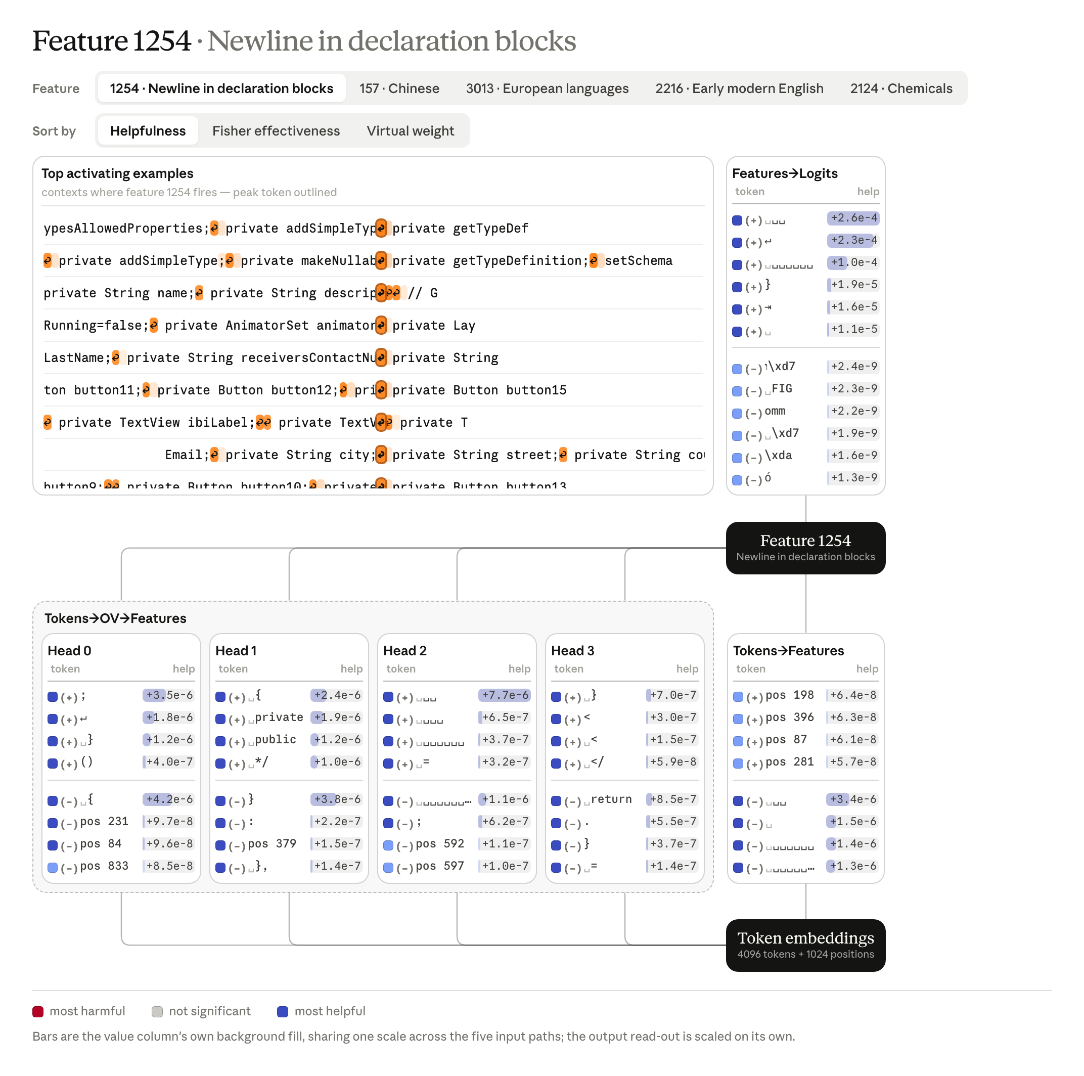
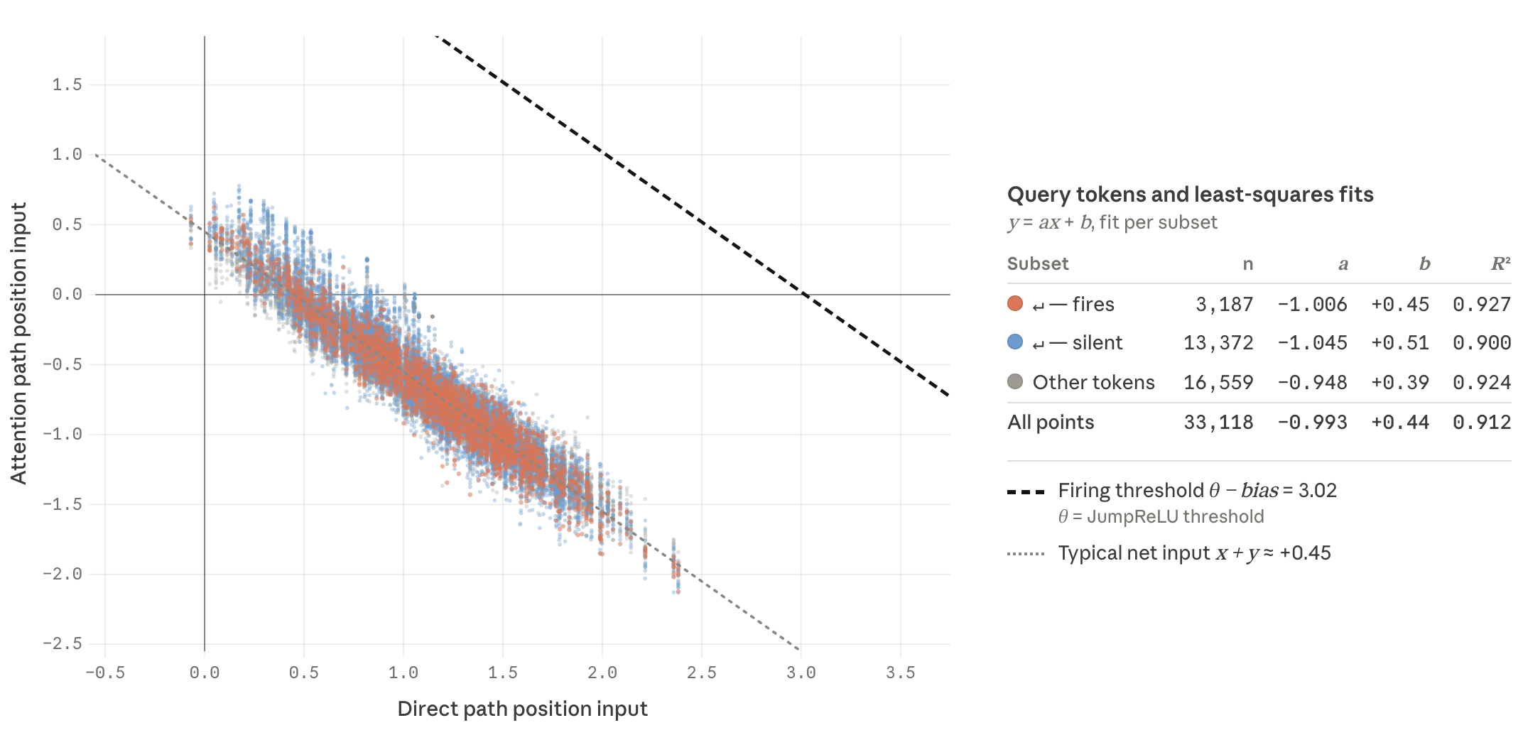
Sorting “IN” connections by effectiveness demotes the harmful “utions” weight and promotes plausible capitalized continuations. Some raw weights already make sense, as for a Chinese-text feature predicting appropriate byte prefixes. Others remain harmful even when effective, including a word-ending feature’s misleading cross-language connections. A newline feature reveals why inhibition matters: large position contributions cancel, attention supplies code-context evidence, and negative direct whitespace weights prevent activation on other whitespace tokens. Thus effectiveness often improves circuit interpretation without perfectly separating helpful and harmful edges.
The effectiveness tail is helpful
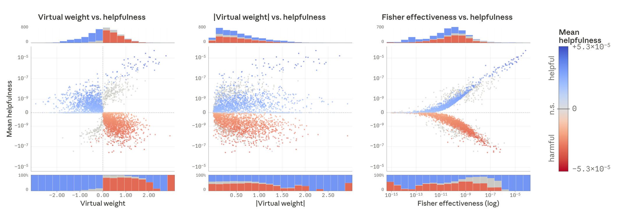
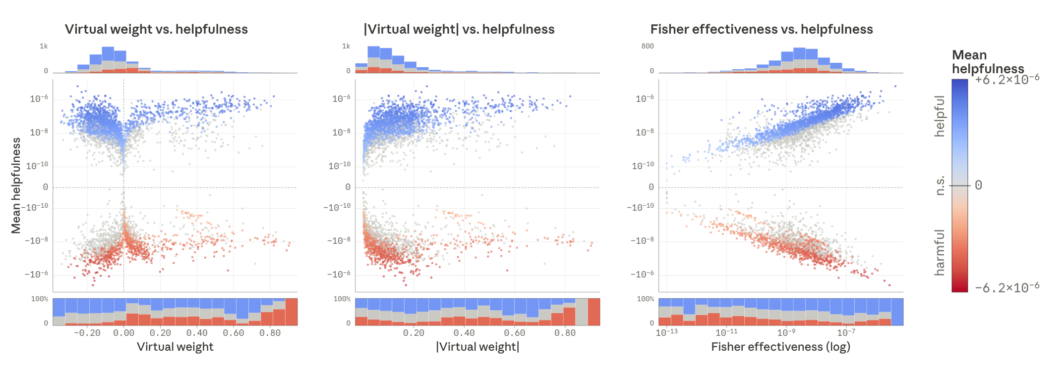
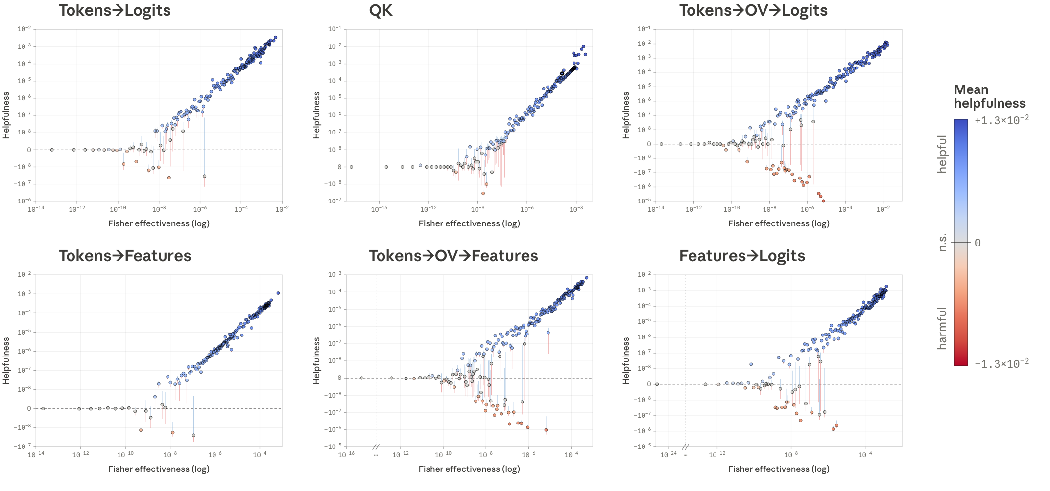
Across 1,111 weights sampled by effectiveness rank, the weakest are nearly inert, the middle contains helpful and harmful connections, and the extreme tail is overwhelmingly helpful. Within each family, the most effective helpful weight exceeds the effectiveness of any sampled harmful one by at least an order of magnitude. This is a sampled empirical pattern, not a universal per-weight guarantee.
The model is still dense in this basis
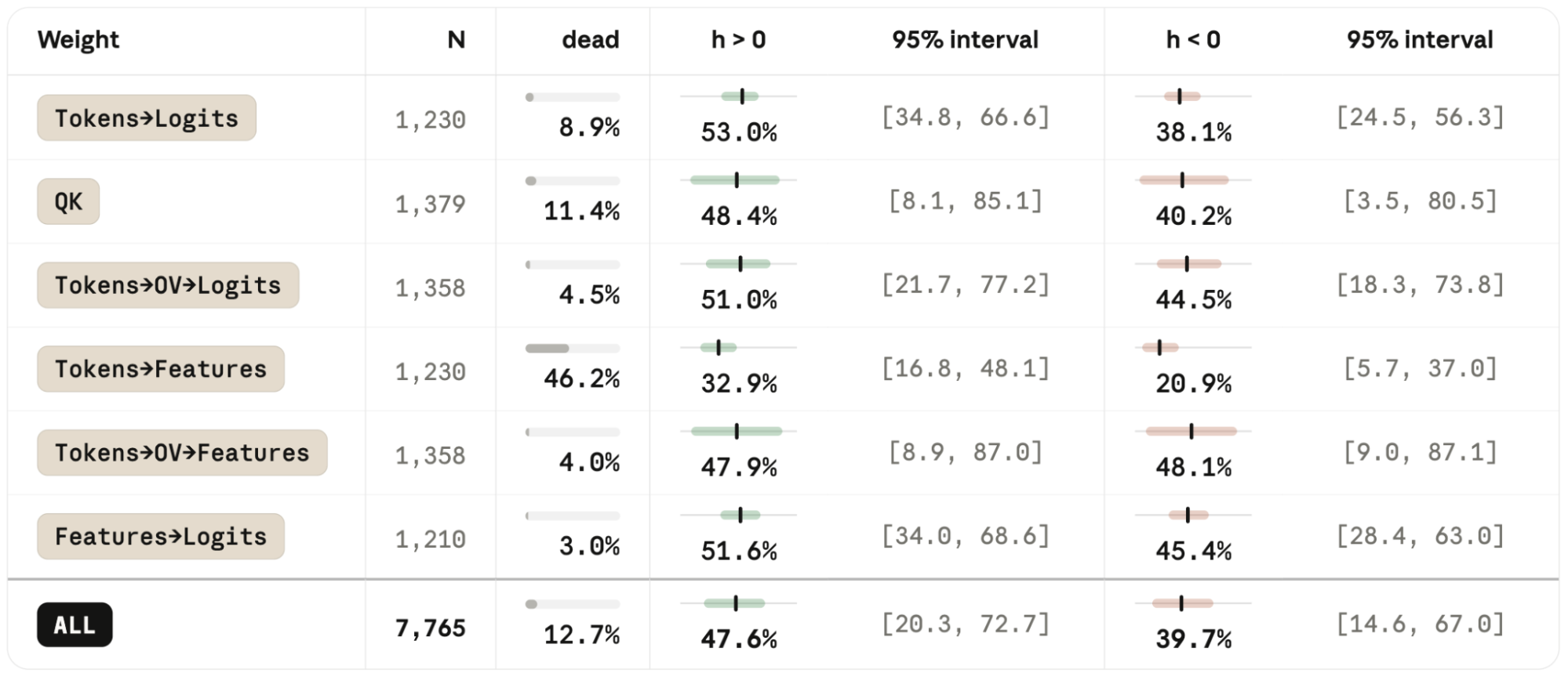
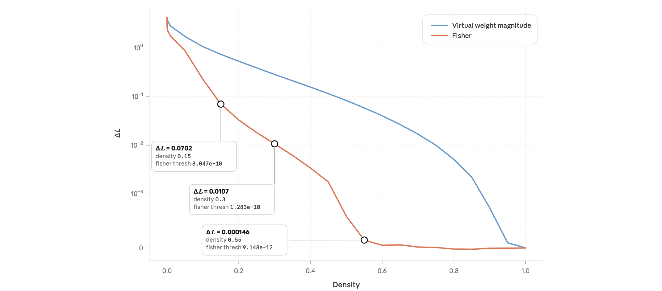
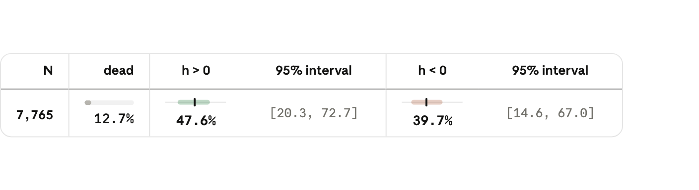
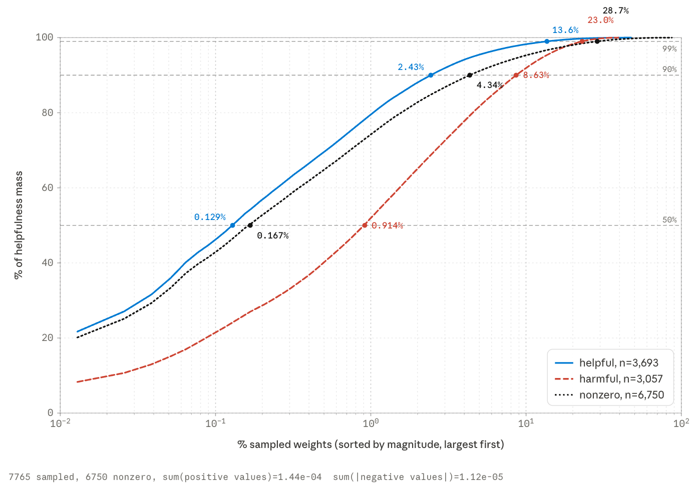
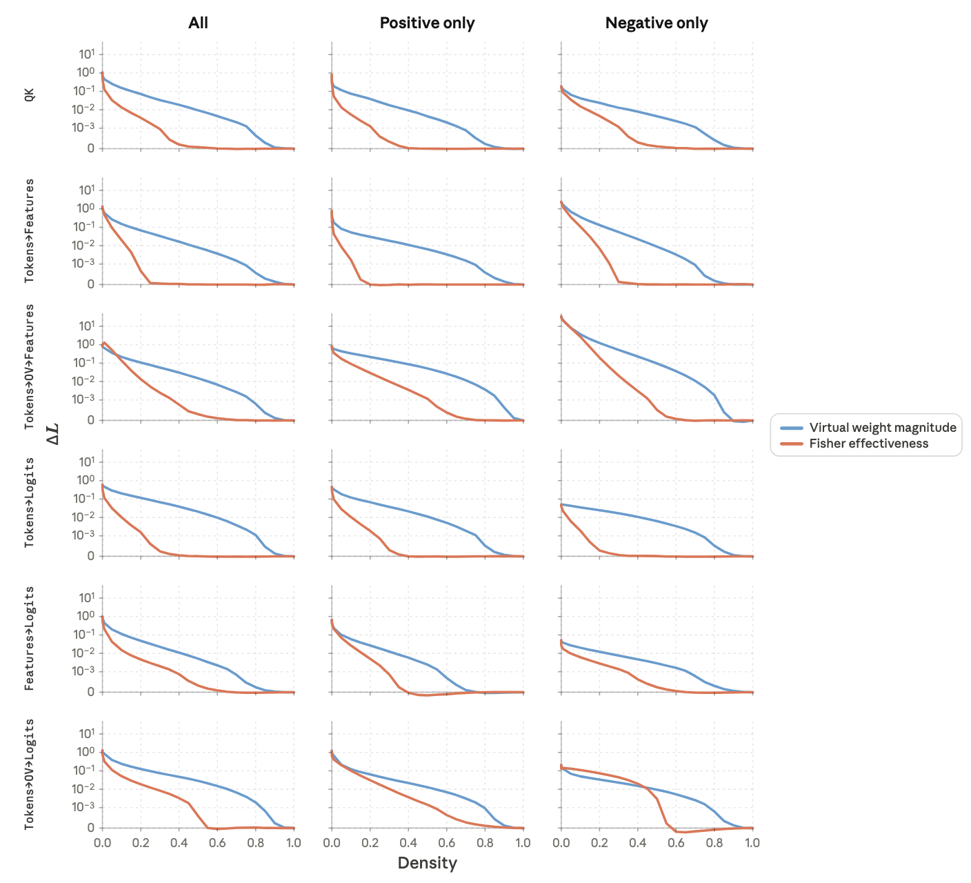
Pruning by effectiveness costs about 0.01 nats at 70% sparsity and less than 0.1 at 85%, substantially outperforming magnitude pruning. Keeping only 1%, approximately the original parameter budget, seriously degrades performance. In a separate 7,765-weight sample, 47.6% have positive mean helpfulness and 12.7% are dead; statistically significant useful weights still occupy tens of percent. Preserving 90% of positive helpfulness mass suggests 2.43% density, but 99% needs 13.6%. These estimates ignore nonlinear interactions between simultaneous ablations.
Discussion
Strong virtual weights are real mathematical connections, but their functional importance depends on the data and competing paths. Effective weights concentrate useful computation, yet this token/transcoder basis remains dense. Better decompositions may matter more than sharper saliency scores. These expensive measurements were feasible in a tiny one-layer model; extending them to frontier models requires scalable proxies. Interference is a concrete consequence of compressed computation, rather than merely an artifact of imperfect feature extraction.
Appendix
The appendices retain training specifications, exact virtual-model construction, effectiveness and helpfulness derivations, and all distributional diagnostics.
Acknowledgments
The authors acknowledge the Anthropic interpretability team and organizational and review support.
Citation Information
The original attribution record is retained.
Turner, et al., "Characterizing interference weights in a tiny language model", Transformer Circuits, 2026.
@article{turner2026interference,
  author={Turner, Nicholas L. and Wu, Jeffrey and Batson, Joshua},
  title={Characterizing interference weights in a tiny language model},
  journal={Transformer Circuits Thread},
  year={2026},
  url={https://transformer-circuits.pub/2026/workspace/index.html}
}
Training details
Transformer and transcoder settings are detailed separately below.
Transformer
The decoder-only transformer has one layer, four 64-dimensional attention heads, a width-1,024 ReLU MLP, and no normalization or biases. Fixed sinusoidal positions and a truncated 4,096-token tokenizer are trained on English/code from Common Corpus. Nine shards train and a tenth evaluates. Adam processes about 98 million unique tokens in 11,933 steps without repetition; training loss falls from 8.93 to about 3.33 nats and is still decreasing.
Transcoder
The single-layer transcoder predicts the MLP output from its input with 4,096 JumpReLU features. Reconstruction loss plus decoder-weighted L1 sparsity trains for 100,000 batches of 16,384 activations, about 1.64 billion samples from repeated corpus passes. Sparsity ramps to 2.0; Adam starts at learning rate 2×10⁻⁵ and decays during the last 20%. Input centering and scaling are folded into final weights.
ACETYLCHOLINE example pairplot
The full pairplot compares direct, attention, and MLP logit contributions against all candidate continuations of ACETYLCHOLINE.
Details of the virtual weight model
The expanded model is an exact forward-pass replacement when its separately carried transcoder error is included.
The [token, position] encoding.
Concatenate token and position one-hot vectors into 5,120 coordinates, with exactly two active entries. Multiplying the original embeddings into downstream matrices gives equivalent fixed virtual weights because the transformer has no normalization.
Moved tokens.
Attention-weighted sums of the concatenated token/position vectors form a moved-token representation. Fixed OV matrices act on those vectors.
Equation
The transcoder error term.
The difference between the real MLP output and its transcoder prediction is unembedded and added back to logits. This correction remains unscored in every effectiveness and helpfulness calculation.
Full schematic diagram
The schematic connects each expanded weight family and its correction term to the original transformer.
Fisher effectiveness computation for all paths
The common Fisher quadratic form uses a weight’s vector of logit attributions and the output softmax information matrix. Path-specific approximations follow.
Equation
Paths to logits
For paths directly into logits, only one attribution entry is nonzero. The quadratic form reduces to the squared source-weight contribution multiplied by the target probability and one minus that probability.
Equation
Paths to features
For paths into features, attribution combines the feature-activation change with its decoder’s logit effects. A counterfactual JumpReLU evaluation captures gate flips and inhibition that frozen-gate gradients miss. The full probability-weighted variance works better than a diagonal-only approximation.
Equation
QK weights
For QK weights, derive the attention change from ablating a score, then propagate it to logits. Repeated appearances of the same token are treated independently, and feature gates are held fixed. These approximations mean the result is not an exact joint counterfactual for all uses of a QK weight.
Shifting attention patterns
The retained derivation expresses how changing one score rescales the softmax partition function and all attention probabilities. A shared ratio combines the affected position and every other position into one formula.
Equations
Writing the attribution vector
Sum the attention shift against direct logit effects and feature-mediated effects. Attention redistribution between positions with identical downstream effects cancels. For tractability, indirect feature contributions omit cross-feature covariances, and covariance between direct and indirect routes is also dropped.
Equations
Computation
All scores average over 2²⁹ training-corpus tokens, with pruning evaluated on disjoint test contexts. Factored activation statistics permit streaming accumulation for all weights; counterfactual calculations exploit source sparsity. Shards are summed before normalization.
Helpfulness computations for weight families targeting the logits
For weights into one logit, the exact softmax partition-function ratio gives the ablation loss change, plus a target-logit correction when that logit is the true answer. Unlike the QK approximation, repeated attended occurrences can be combined exactly because they affect the same logit.
Equations
Single weight helpfulness histograms
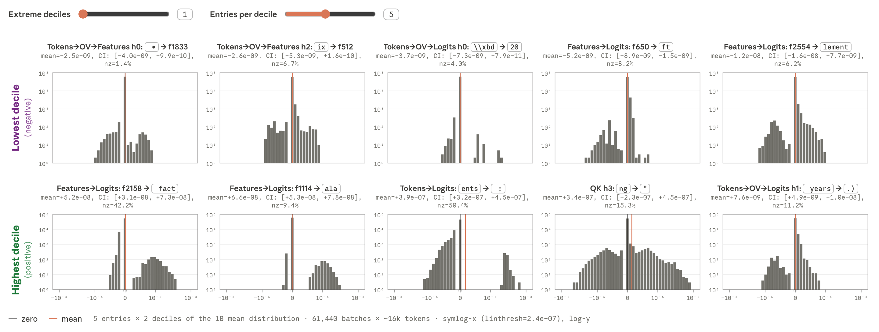
Per-batch helpfulness distributions for sampled weights are broad and often cross zero even when their overall means have a confident sign. Each batch contains 16,384 tokens.
Mean helpfulness histograms
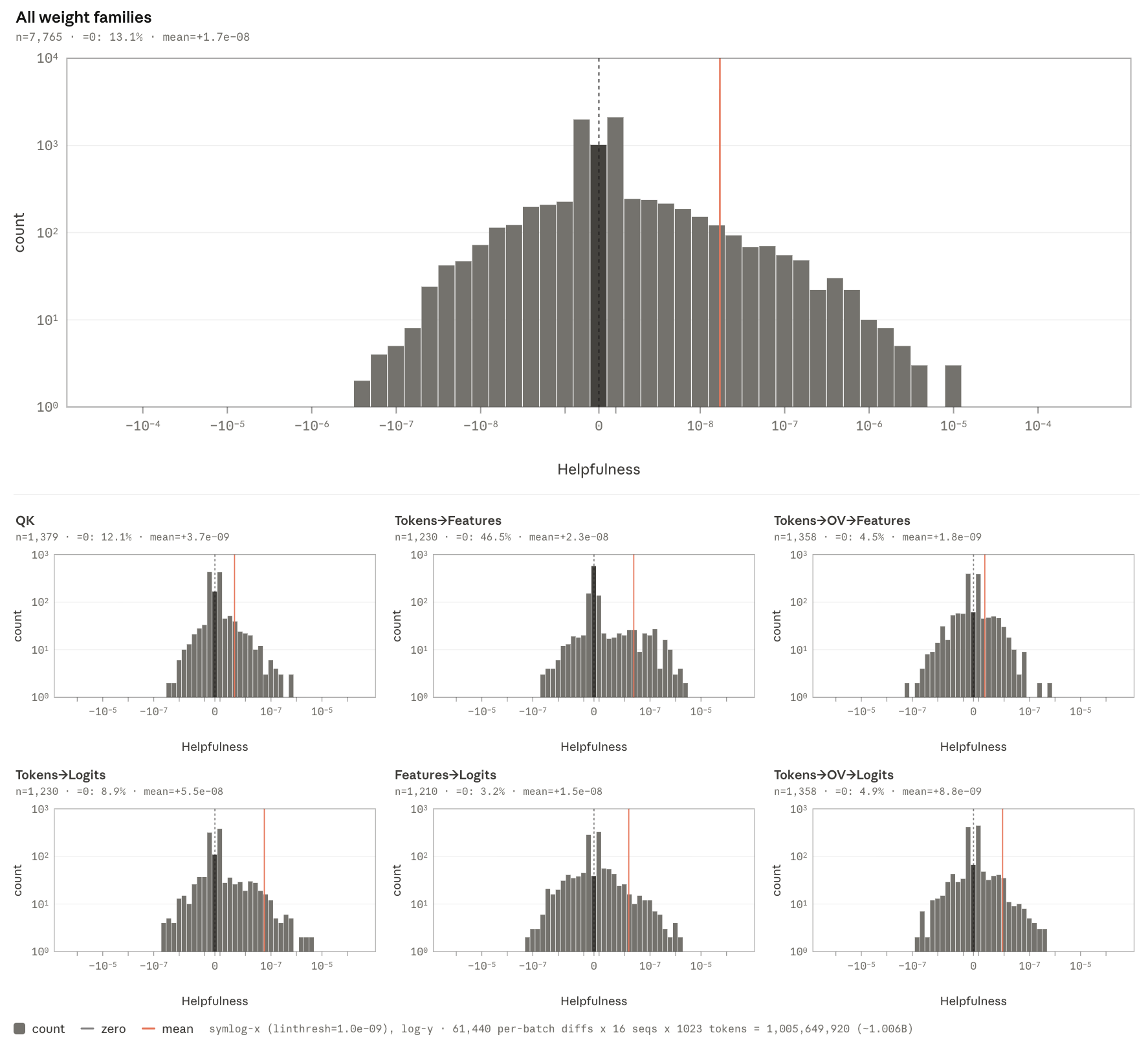
Mean helpfulness across 7,765 weights is concentrated near zero, approximately symmetric, and slightly heavier on the useful side.
Sampled mean-helpfulness CDF
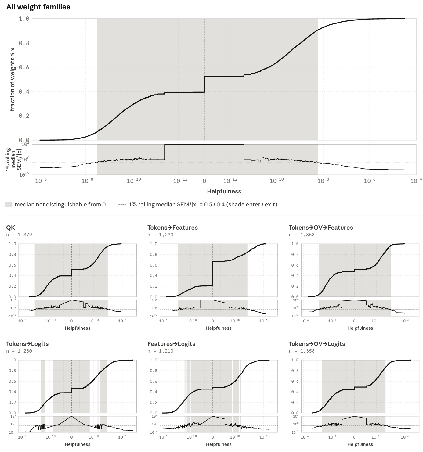
The cumulative helpfulness distribution marks regions where means cannot normally be distinguished from zero using nearby standard-error estimates.
Helpfulness mass distribution
Positive, negative, and total absolute helpfulness mass are accumulated separately; percentages refer to the entire sample. Of 7,765 weights, 6,750 have nonzero helpfulness. Positive mass totals 1.44×10⁻⁴ versus 1.12×10⁻⁵ for negative magnitude.
Fisher effectiveness CDF
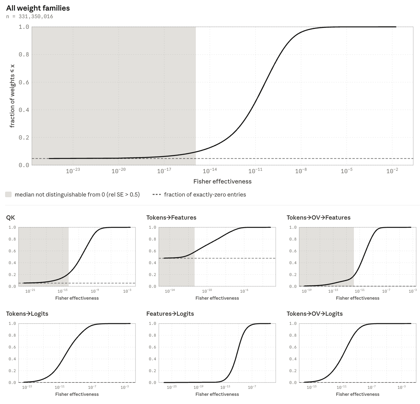
The effectiveness cumulative distribution similarly marks a local uncertainty region around zero.
Fisher mass distribution
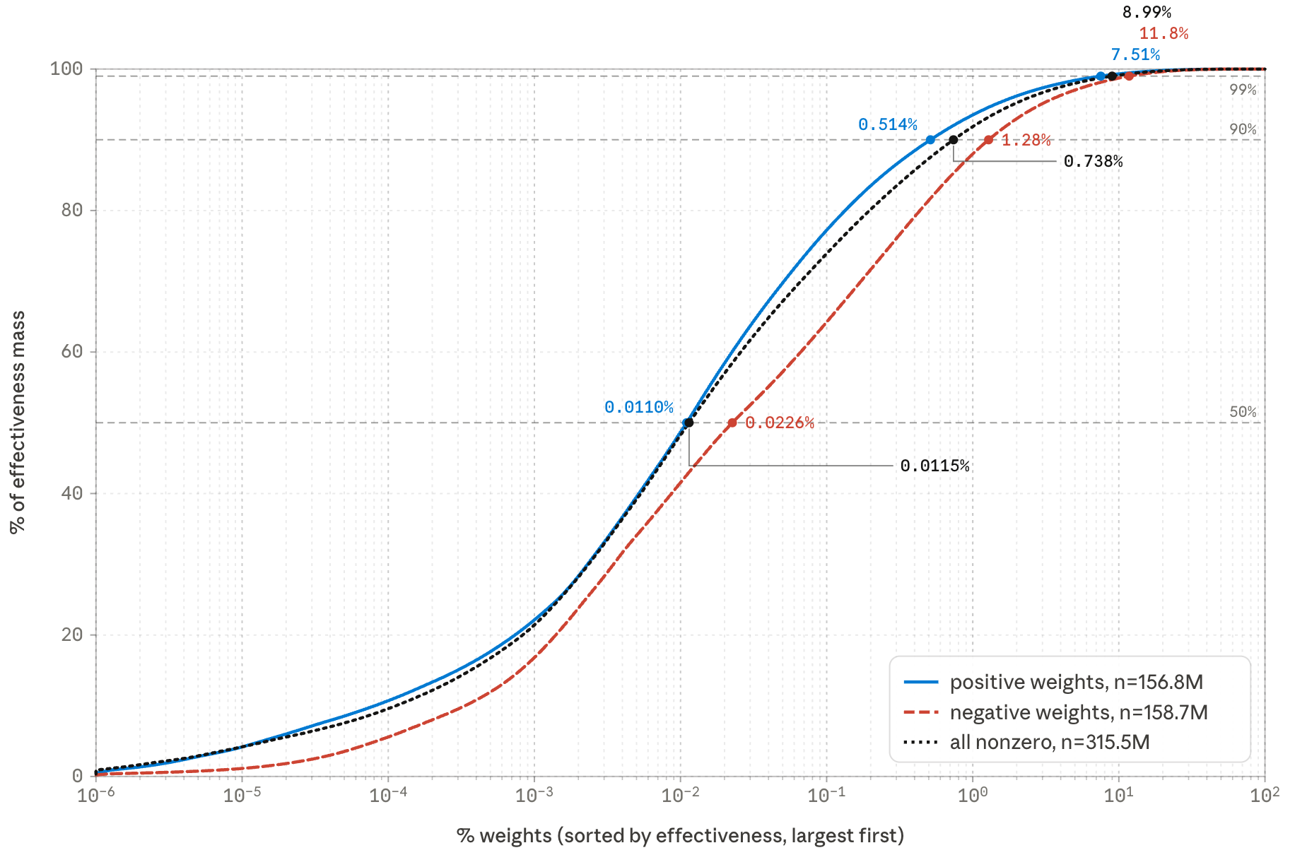
Across all 331,350,016 virtual weights, 315,487,613 have nonzero measured effectiveness. Total effectiveness is 3.62 for positive weights and 1.59 for negative weights; these are unsigned effectiveness contributions grouped by weight sign.
Fisher effectiveness vs. expected attribution
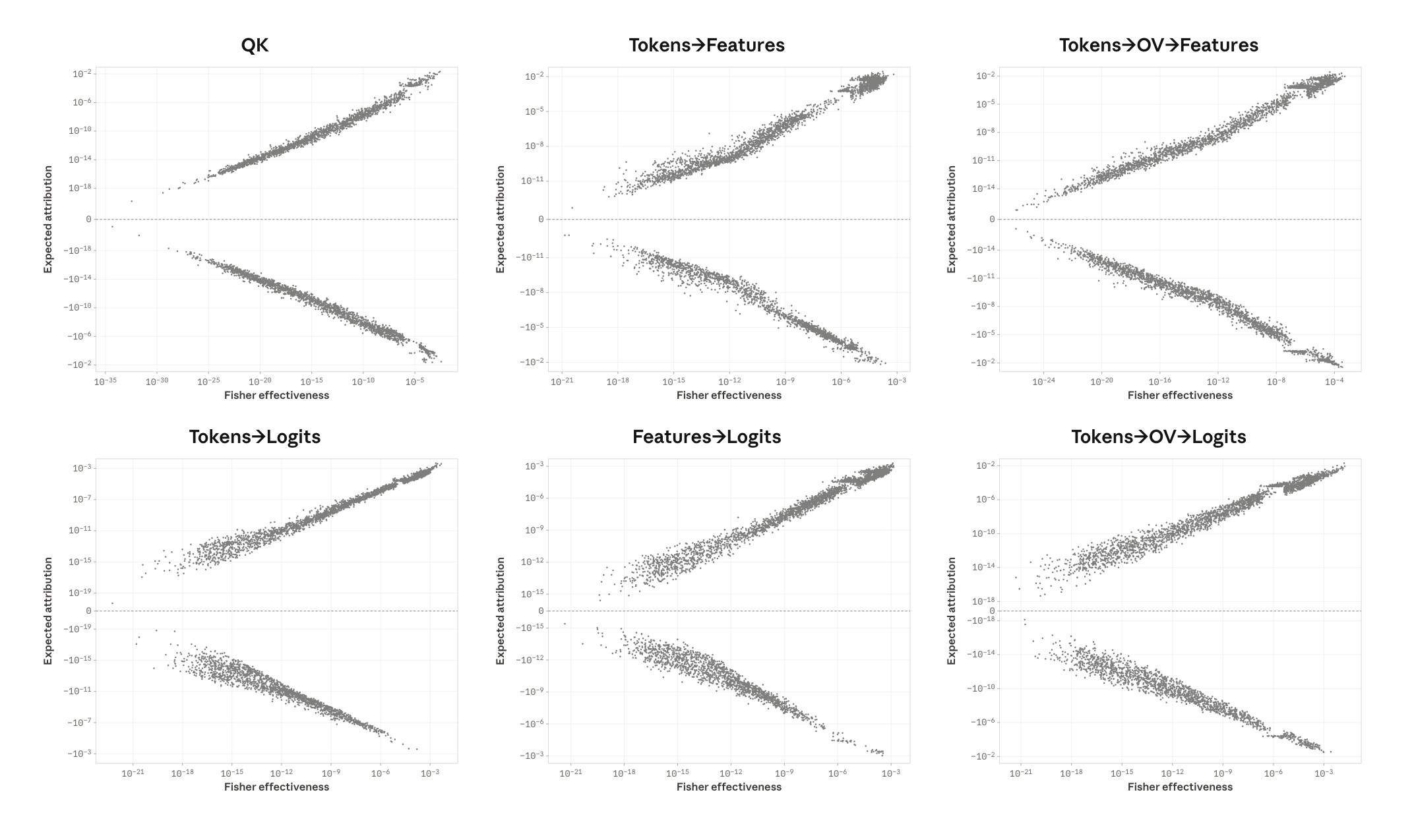
About 27,000 sampled points compare Fisher effectiveness with an updated expected-attribution proxy. Counterfactual feature attribution and linearized output/QK attribution make this a close but modified comparison with the earlier ERA metric.
Feature 1254 position input
The newline feature’s direct and attention-mediated position inputs nearly cancel, leaving only a small fraction of its activation threshold.
Virtual weight magnitude vs. helpfulness
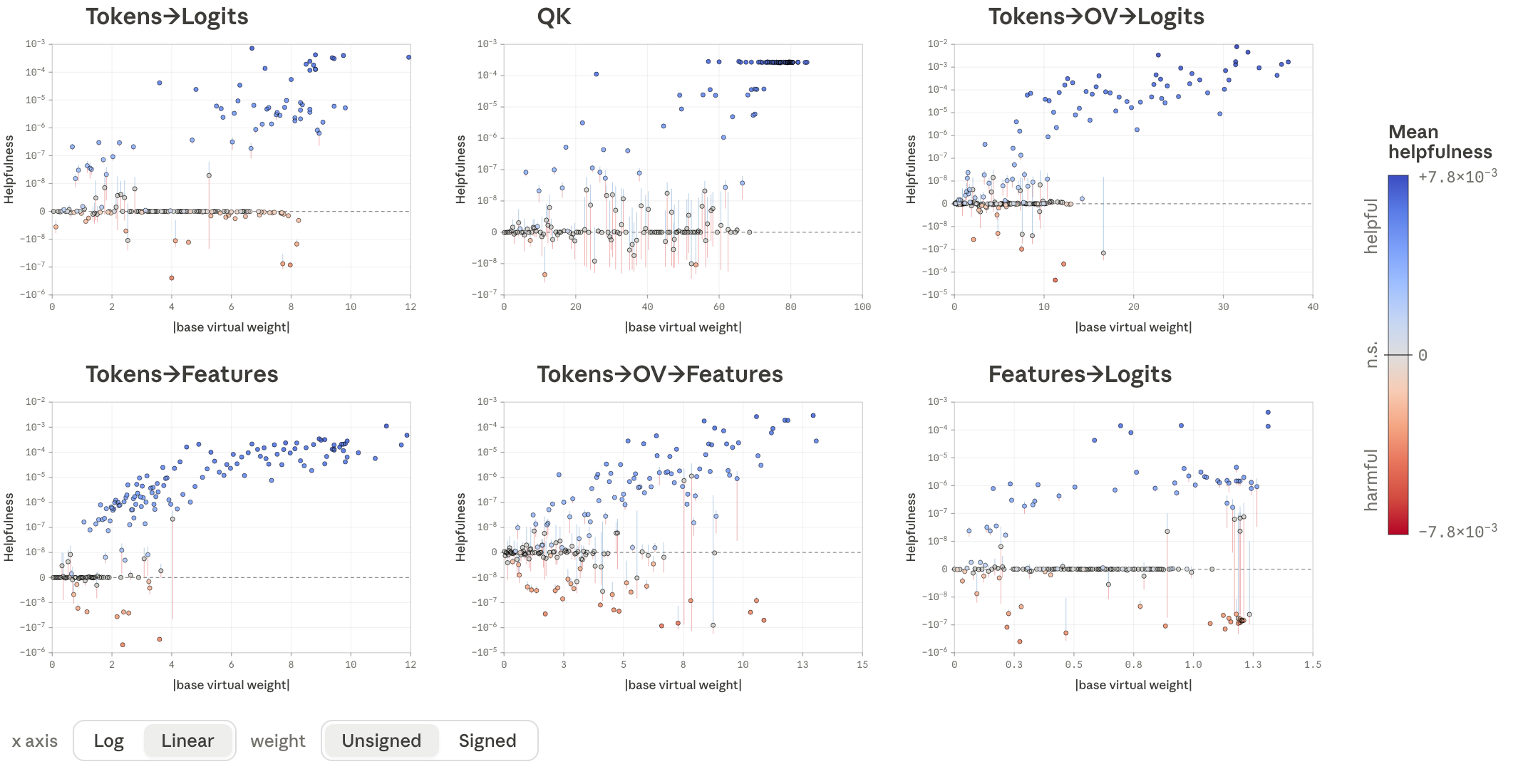
Raw virtual-weight magnitude does not show a consistent separation between the strongest helpful and harmful weights across families.
Threshold eval plots and CDFs for each weight
Family-specific pruning curves separate positive and negative weights. Negative feature-to-logit weights are the stated exception to the general advantage over magnitude pruning.
ROPE plots
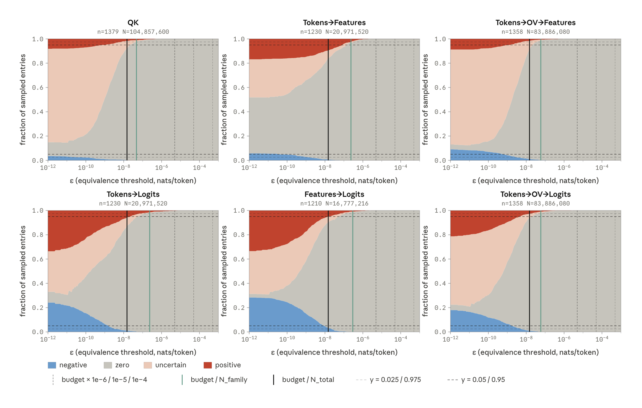
A region of practical equivalence distinguishes statistically detectable changes from meaningful loss effects. A weight is useful or harmful only when its whole confidence interval lies beyond the chosen tolerance; intervals fully inside are practically zero, and the remainder are uncertain. The comparison uses the model’s roughly 4.94-nat gain over uniform prediction as one scale, but choosing a practical tolerance remains application-dependent.
Full helpfulness table
The complete helpfulness classification expands the main-text proportions and preserves the uncertainty accounting.